The purpose of this page is just to serve as todo or scratch pad for the development project and to list and share some ideas.
After making changes to the code and/or documentation, this page should remain on the website as a reminder of what was done and how it was done. However, there is no guarantee that this page is updated in the end to reflect the final state of the project
So chances are that this page is considerably outdated and irrelevant. The notes here might not reflect the current state of the code, and you should not use this as serious documentation.
Replicate functionality of MNE software
Objectives
to replicate the functionality of MNE software in FieldTrip. The same functions will be usable for researchers at the Donders Institute without learning how to use a new software (MNE). Therefore, the project is focusing on adapting the functions to the requirements and to technical facilities of this institute.
What is MNE?
MNE is a software package that is developed in the A. A. Martinos Center for Biomedical Imaging and it is used for preprocessing averaging EEG and MEG data and for constructing cortically-constrained minimum-norm estimates. The software is written on C and MATLAB, and a MATLAB Toolbox related to the software is also provided. The software depends on anatomical MRI processing tools provided by the FreeSurfer software.
What is FreeSurfer?
FreeSurfer is a software for the study of cortical and subcortical anatomy. Among other functions, it constructs models of the boundary between white matter and cortical gray matter as well as the pial surface. The surfaces can be inflated or flattened for improved visualization. The surfaces can be also used to constrain the solutions to inverse EEG and MEG problems.
Overview
Step 1
Goal
- to define which are the equivalent FieldTrip functions of the MNE functions. If it is necessary, FieldTrip functions will be adapted.
- to define how it is possible to switch from MNE to FieldTrip at each processing level
- this also involves writing the read/write functions so that data can be exchanged
Step 2
Goal
to test the equivalence of the two software pipelines on a simulated dataset
MNE Pipeline
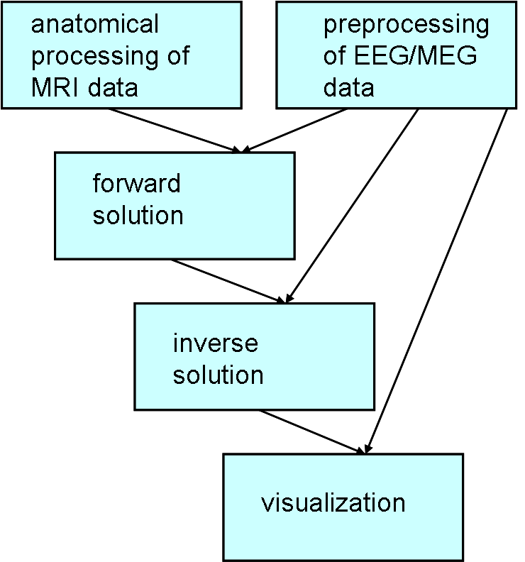
The pipeline of the MNE analysis can be divided into 5 bigger step
- Anatomical processing of MRI data. MNE software is using the output and some of the functions of FreeSurfer (FS).
- Preprocessing of EEG/MEG data. MNE calculates also the average and the noise-covariance matrix.
- Calculation of the forward solution.
- Calculation of the inverse operator.
- Visualization.
The last three steps are using the outputs from processing of anatomical and electrophysiological data.
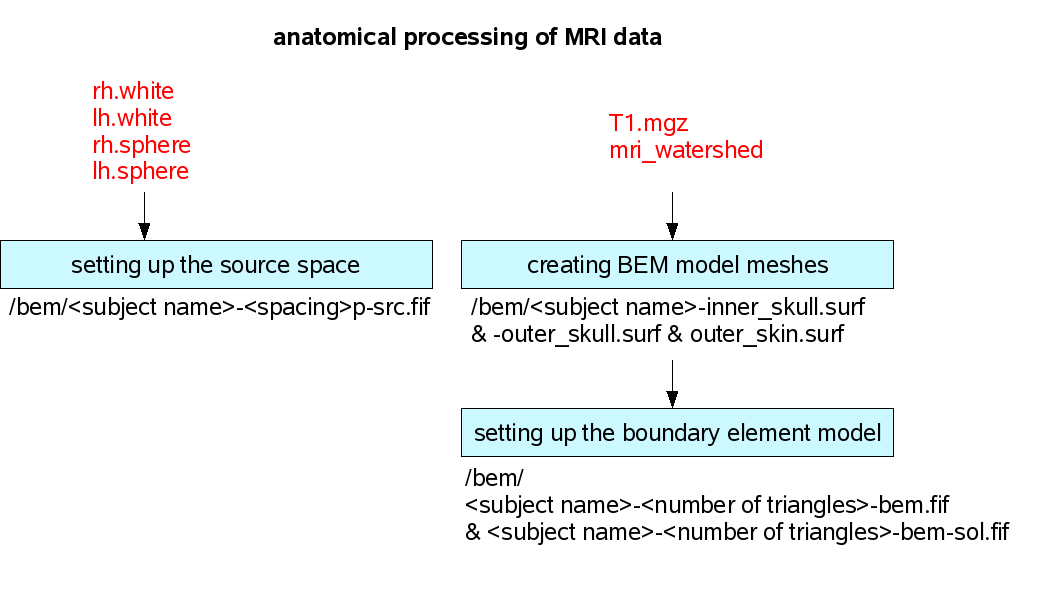
1. Anatomical processing
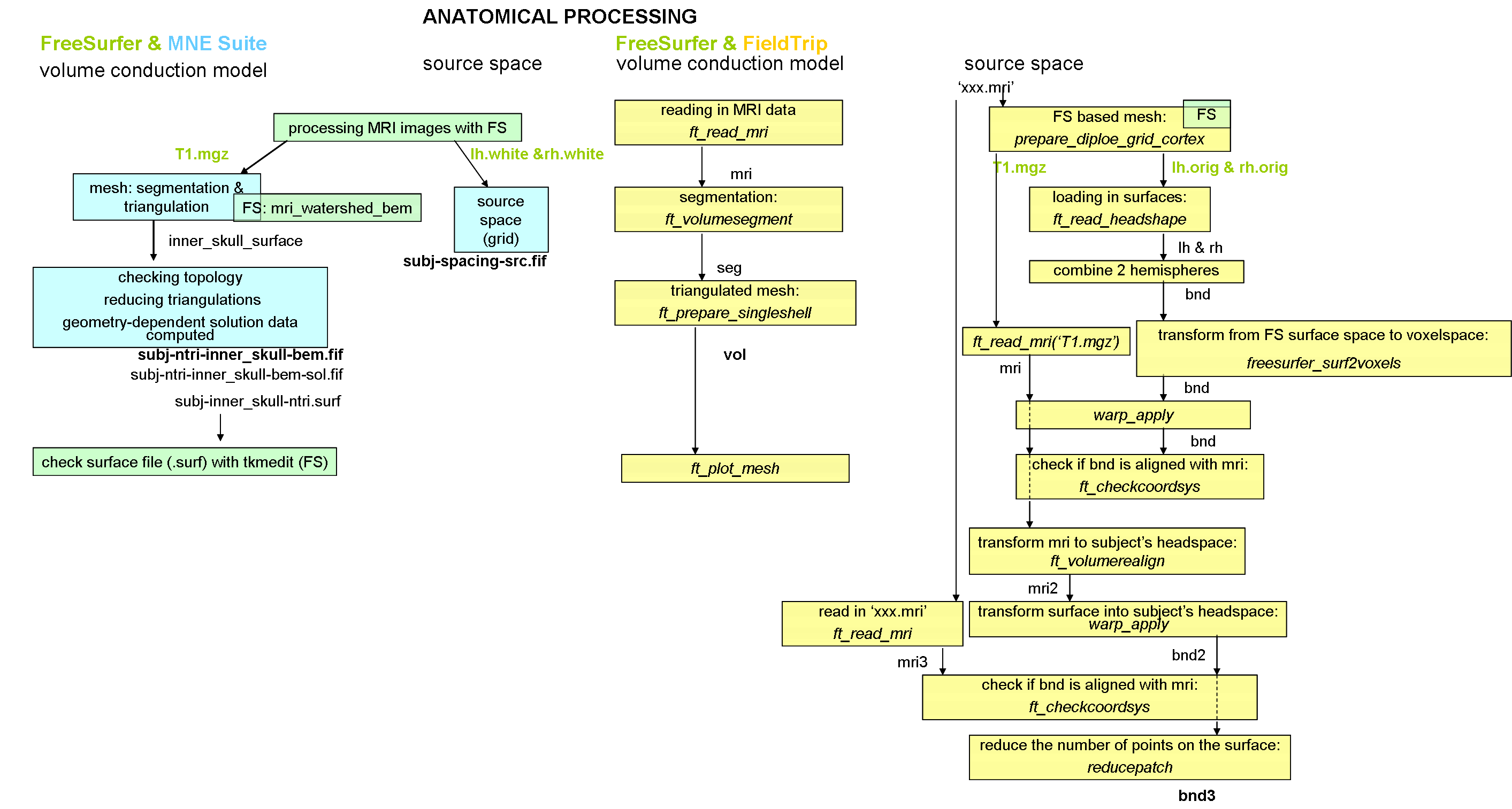
The first part of anatomical processing of the MRI data is done by the FreeSurfer program. MNE is using the output of this program and one of the FS functions to create head shapes with the boundary element method (BEM) and to set up the source space for the forward solution. The next figure shows the filenames (with red) that were created by FS and MNE is using them for input. When MNE is creating the BEM model meshes it is using a function (mri_watershed) from FS. Therefore, the FS has to be set up before running this MNE function.
First, one should run FS for creating the input files for MNE.
Using FS
The recommended workflow of FS has three automatized processing steps. But first of all, the data has to be imported.
Sourcing FS, setting up environmental variables, importing data
Codes are included that works on Linux (with bash type of shell) and on Siemens DICOM data (raw data files with .ima extension).
environmental variables have to be set up:
export FREESURFER_HOME=
This code will recognize the first xxx.ima file in the directory of the anatomical data, and it will find the other files automatically. It will create a directory under $SUBJECTS_DIR with the given subject’s name. It will also create more directories. One created directory is named orig under $SUBJECTS_DIR/<subject’s name>/mri where there will be a 001.mgz file (containing all anatomical data) that will be used as input for further processing. If there were more scanning runs of the same subject, other .mgz files will be created (001, 002… etc.) But I do not know if more scans of the same subjects are automatically recognized. :
autorecon 1
recon-all -autorecon1 -subjid <subject's name>
This figure shows the processing steps done by -autorecon1 when there is only one scanning run of one subject is available. The input and output file names are shown also for each step.
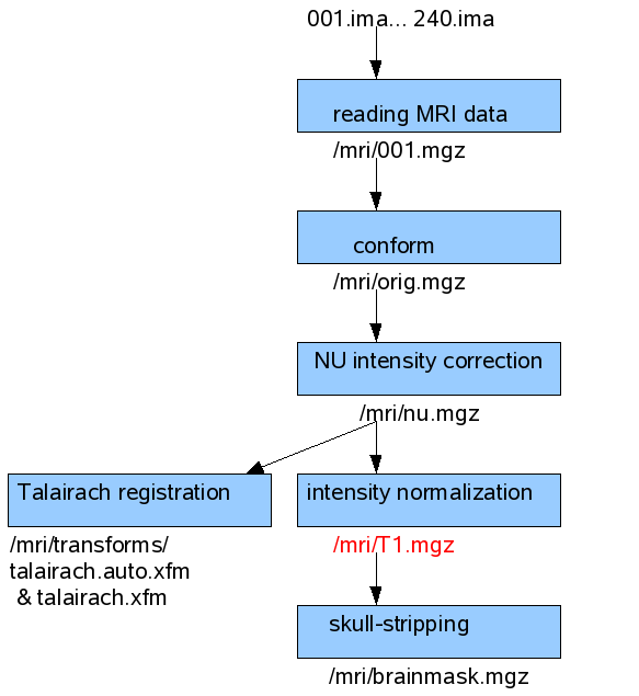
This first processing step takes around 1,5 hour.
First, it is averaging the multiple scanning runs together if they exist (output: $SUBJECTS_DIR/<subject’s name>/mri/rawavg.mgz), corrects small motions between them and conforms the data to 256 voxels (1mm size) for all directions (output: $SUBJECTS_DIR/<subject’s name>/mri/orig.mgz).
Then, a non-parametric non-uniform intensity normalization (N3) corrects for intensity non-uniformities (output: $SUBJECTS_DIR/<subject’s name>/mri/nu.mgz). Next, talairach transformation is computed (from nu.mgz) using MNI305 atlas, and outputs the transformation into $SUBJECTS_DIR/<subject’s name>/mri/transforms/talairach.auto.xfm and talairach.xfm.
Then, it performs an intensity normalization (intensity of all voxels are scaled) and gives the output $SUBJECTS_DIR/<subject’s name>/mri/T1.mgz. This is the volume that is used by the interactive analysis tool of MNE, mne_analyze where the MRI Viewer is using the T1.mgz volume together with the FreeSurfer tkmedit user interface. The tkmedit shows the MRI volume index and the Talairach coordinates. T1.mgz is also used as input for MNE for creating BEM meshes.
Last, the mri_watershed program is running that finds the boundary between the brain and the skull (output: $SUBJECTS_DIR/<subject’s name>/mri/brainmask.auto.mgz and $SUBJECTS_DIR/<subject’s name>/mri/brainmask.mgz).
When this step is ready, it is possible to check if the Talairach transformation and the skull stripping are correct.
tkregister2 --mgz --s <subject's name> --fstal
tkmedit <subject's name> brainmask.mgz -aux T1.mgz
autorecon 2 and autorecon 3
The next two steps are creating the surfaces (white, pial and inflated).
recon-all -autorecon2 -subjid <subject's name>
This step takes around 10-12 hours. The outputs of this processing step among others are the white surfaces (left and right hemisphere) that is used by MNE to set up the source space. It is possible to check and correct the white and pial surfaces after they were constructed. An example code for the check:
tkmedit<subject's name>wm.mgz rh.white -aux brainmask.mgz aux-surface rh.white
For further instructions, read http://surfer.nmr.mgh.harvard.edu/fswiki/RecommendedReconstruction
This figure shows the processing steps that happens when -autorecon2 is running. Not all of the output files are shown, and many of the processing stages could be divided into more individual FS functions. But I tried to add those output files that are used as input of later processing stages. The red file names are used later by MNE. The last step (green) belongs to -autorecon3.

In the first stage (automatic subcortical segmentation) the volume is further normalized based on a GCA (gaussian filter array) model.
Then, a second (major) intensity correction is performed again. Now, the intensity correction is done on a volume from which the skull has been removed (compared to the intensity correction in -autorecon1.
In the next stage (white matter segmentation), the white matter is separated from everything else.
Then (cutting and filling), the mid brain is cut from cerebellum and the hemispheres are cut from each other. The left hemisphere is binarized to 255, the righ hemisphere to 127.
Next (tessellation), the surface is created by covering the filled hemispheres with triangles.
Finally, the pial, white and inflated surfaces are created. The white surface is created that so that it follows the white-gray intensity gradient as found in the T1 volume. The pial surface is created by expanding the white surface so that it follows the gray-CSF intensity gradient. (for a bit more detailed description, see http://surfer.nmr.mgh.harvard.edu/fswiki/recon-all)
In order to run the last processing stage of the figure (spherical inflation) one should run the third automatic reconstruction step of FS.
recon-all -autorecon3 -subjid<subject’s name>
This step requires also quite much time (around 8-10 hours). It inflates the surface into sphere. But it does more than only the spherical inflation. However, as far as I know, MNE is using only the output of this first processing stage of -autorecon3. Therefore, maybe it would be useful to run only this stage instead of the entire -autorecon3. It takes around 3-4 hours. :
mris_sphere rh.inflated rh.sphere
mris_sphere lh.inflated lh.sphere
Anatomical processing with MNE
Setting up MNE
export MNE_ROOT=<MNE directory>
cd $MNE_ROOT/bin
. ./mne_setup_sh
MNE requires to set up the same environmental variables as FS. It is because MNE will look for the MRI data that is processed by FS (therefore, it will look for directories that are made by FS). Therefore, SUBJECTS_DIR environmental variable should refer to that directory where the anatomical data is (pre-processed by FS), and SUBJECT should refer to the sub-directory of SUBJECTS_DIR where the anatomical data is from the person whose data is analyzed. Besides the SUBJECTS_DIR, there is usually an other directory, named EEG or MEG where the electrophysiological data is. It should have a sub-directory with the data of the person whose data is analyzed (named the same as SUBJECT). For example:
<MNE ANALYSIS DIR>/subjects/<subject's name>: contains the output from FS

<MNE ANALYSIS DIR>/MEG/<subject's name>: contains the electrophysiological data

export SUBJECTS_DIR=<MNE ANALYSIS DIR>/subjects
export SUBJECT=<subject's name>
Setting up the source space
mne_setup_source_space --ico -6
MNE is using a distributed inverse solver for EEG/MEG source estimation. Therefore, it discretize a source space into locations on the cortical surface. At a later stage, the desired solution will be computed by finding a source distribution with a minimum overall energy that depends on all sources in the source space.
This stage creates a decimated dipole grid on the white matter surface, and saves this source space file in fif format. The location of the sources in the source space are expressed in “surface RAS coordinates” in the fif files. (The origin of this coordinate system is at the center of the conformed FreeSurfer MRI volumes and the axes are oriented along the axes of this volume.)
This script is looking for a surface as input in the $SUBJECTS_DIR/$SUBJECT/surf directory. By default, the “white” surface is used (rh.white and lh.white). The grid spacing for the source space can be specified in mm. By default, 7mm is used. It is also possible to create the source space using the topology of a recursively subdivided icosahedron or octahedron (by using option –ico). This method is using the cortical surface inflated to a sphere, therefore, it is looking also for the FS surfaces, $SUBJECTS_DIR/$SUBJECT/surf/rh.sphere and lh.sphere as input.
The source space will have triangulation information for the decimated vertices included. In this code, for example, -ico -6 will create a source space with 4.9 mm spacing. If it is specified, it can also compute the cortical patch statistics. It is also possible to use the source space created by using another subject’s data and to morph it to the actual subject.
MNE provides also a support for three-dimensional source spaces and for arbitrarily located source points.
Creating the BEM meshes
In MNE, the calculation of the forward solution is using the boundary-element model (BEM). This requires that surface separating separating regions of different electrical conductivities are tessellated. This software employs triangular tessellation.
mne_watershed_bem
It calculates the segmentation of the MRI data and the triangulation of the relevant surfaces. This code is facilitating the use of watershed algorithm that is part of FS. The program is called mri_watershed. During the processing of MRI data with FS, this program finds the boundary between the brain and the skull. Now, it creates the brain surface triangulation, the inner skull triangulation, the outer skull triangulation and the scalp triangulation.
The input file is in $SUBJECTS_DIR/$SUBJECT/mri/T1.mgz. Here, the surface RAS coordinates system is used, and also the output contains the same. The outputs are: $SUBJECTS_DIR/$SUBJECT/bem/$SUBJECT_brain_surface, $SUBJECT_inner_skull_surface, $SUBJECT_outer_skin_surface, $SUBJECT_outer_skull_surface. However, the next step in MNE will look for these files on a slightly different name: $SUBJECT-inner_skull.surf, $SUBJECT-outer_skin.surf…etc. Therefore, these files have to be renamed. :
When the option –atlas is used, mri_watershed will use atlas information to correct the segmentation.
In addition to using the mri_watershed FS program, the brain MRI volume will be put in bem/watershed/ws in .COR files. And the scalp surface ($SUBJECT_outer_skin_surface) will be converted to fif format (/bem/$SUBJECT-head.fif) with the mne_surf2bem program.Later, mne_analyze will use this file for visualizations.
Setting up the boundary-element model
This step assigns conductivity values to the BEM meshes. The conductivity values can de specified. Without specification, default values are used.
mne_setup_forward_model --homog --surf --ico 4
The –surf option indicates that FS surface files should be used. If –surf is used, –ico is also relevant. It specifies the decimation of the triangulation (and therefore, it is saving computation time). –ico 4 is recommended, it yields to 5120 triangles per surface. –homog species if a single compartment model instead of a three layer model should be used. When –homog is used the input is only the $SUBJECT-inner_skull.surf. This option is recommended when MEG data is analyzed.
This program creates the BEM model geometry specifications (as output
- /bem/$SUBJECT-
-bem.fif (if --homog option is specified) - $SUBJECT-
- .surf for each surface. This can be loaded to tkmedit (FS) to check if the surfaces are correct. - /bem/$SUBJECT-
-bem-sol.fif containing the geometry dependent solution data (optional)
2. Preprocessing of EEG/MEG data
Preprocessing with MNE
In this section, I will go through the steps of preprocessing CTF MEG data.
The following can be done in the preprocessing:
- gradient compensation of CTF MEG data
- filtering
- identifying bad channels
- segmentation
- automatic artifact rejection
- averaging
- noise-covariance estimation
The following files are useful for doing these:
- event file
- channel names
- layout file
- averaging script
- script for covariance estimation
There are two options for processing the data:
- in interactive mode
- in batch mode
Data conversion
The EEG/MEG data has to be converted to .fif format.
mne_cft2fiff --ds /<path to the ds directory>/xxx.ds --fif<subject's name>_raw
Identifying bad channels and checking filters
All options that are available in batch mode, are also available in interactive mode. In interactive mode, one can also look at the raw data at each channel and therefore, it is possible to identify bad channels. After averaging, the averages can be seen also in the interactive mode if the appropriate layout file is available.
It is useful if one calls the interactive mode from the directory where the raw data file is stored. In this case, the name of the trigger channel is different as default (STI 014), so the name of the trigger channel has to be specified otherwise the data can not be seen. It is done with the –digtrig flag.
cd<path to directory>/MEG/<subject's name>mne_browse_raw --digtrig STIM\
Averaging in batch mode
mne_process_raw --raw<subject's name>_raw.fif --digtrig STIM --events<event file>.fif --projoff --ave<averaging script>.ave
Noise-covarinace estimation in batch mode
mne_process_raw --raw<subject's name>_raw.fif --digtrig STIM --events<event file>.fif --projoff --cov<script for covariance estimation>.cov
Looking at the averages
cd<path to directory>/MEG/<subject's name>mne_browse_raw --digtrig STIM\
Go to File in the menu and choose: Open Evoked. Choose the fif file that containes the averaged data. Then go to Adjust in menu, choose: Layouts. Choose the appropriate layout file. And go to Windows in menu and choose: Show Averages.
3. Forward solution
Align coordinate frames
Before calculating the forward solution, the MRI and the MEG data has to be aligned by identifying the fiducials (left AP, right AP and nasion). The alignment is done in an interactive mod
cd <path to directory>/MEG/<subject's name>
mne_analyze
Forward solution
mne_do_forward_solution --mindist5 --spacing oct-6 --bem<subject's name>-5120-5120-5120-bem.fif --meas<file with averages>.fif
4. Inverse solution
mne_do_inverse_operator --fwd<file containing the forward solution>.fif --depth --loose 0.2 --meg
5. Visualization
cd <path to directory>/MEG/<subject's name>
mne_analyze
FieldTrip Pipeline
This is a general pipeline about how to do source analysis based on minimum-norm estimate.
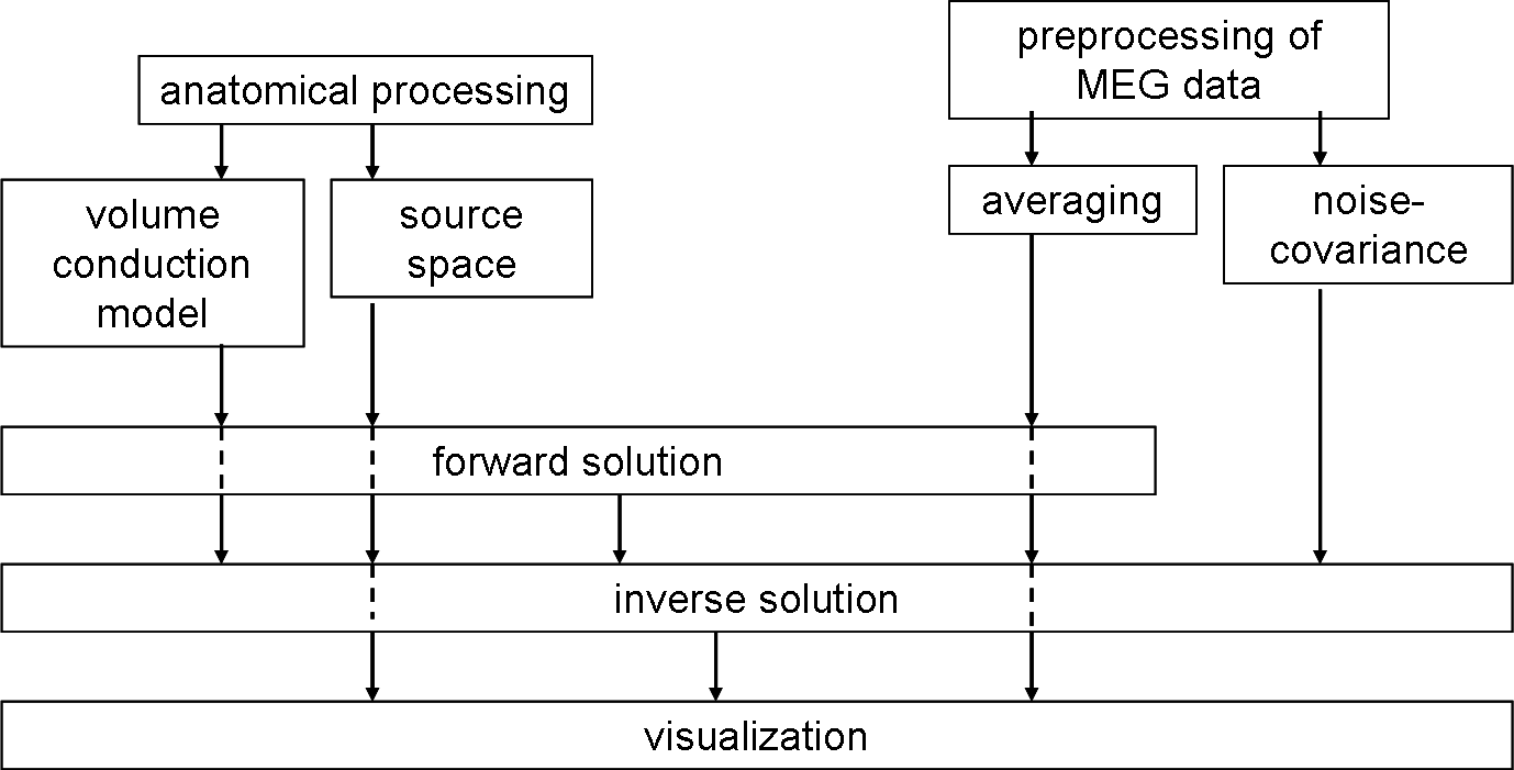
Anatomical processing:MEG
The following figure shows the MNE and FS and FT pipeline of anatomical processing.
–0)
:!: Creating source space in FieldTrip has been tested only on MRI data with .mri extension.
In FieldTrip, the volume conductor model and the source space are both should aligned to the CTF head-coordinate system. The function ft_checkcoordsys helps to control it.
In MNE Suite, the alignment and the coordinate transformation happens only just before calculating the forward solution (when the volume conductor model and the source space have been already set up.)
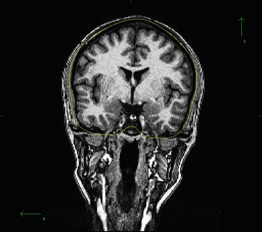
Plotting innerskull from MNE
innerskull = ft_read_headshape(<path to directory>/subjects/<subject's name>/bem/<subject's name>-inner_skull-5120.surf');
ft_plot_mesh(innerskull);
Innerskull in tkmedit
I could load in only the sub10_inner_skull_surface file (output of mne_watershed_bem) in tkmedit overlayed on the T1.mgz.
Plotting vol from FT
ft_plot_mesh(vol.bnd);
Plotting bnd3 from FT
ft_plot_mesh(bnd3);
Anatomical processing: EEG
Reading in data
FieldTrip is MATLAB based processing tool. Therefore, MATLAB is needed to run its functions. The preparation before starting FieldTrip is that the downloaded FieldTrip has to be added to the MATLAB path.
Function ft_read_mri can read in MRI data in many formats. Look at Supported data formats. The .mgz files (freesurfer) format is not listed yet, but the function can read in also that volume.
mri=ft_read_mri(<path to directory>/T1.mgz');
If you want to work with the .ima images, you have to put only the name of first image file into the path.
mri=ft_read_mri(<path to .ima directory>/XXX.ima');
Realignment
At this moment, the segmentation algorithm works only with mri data that is aligned to a CTF-based or SPM-based coordinate system. Therefore, first the function ft_volumerealign should be run that makes the transformation matrix of the mri data correspond to the CTF coordinates system. For this, one should identify the nasion, the LPA and RPA (left and right pre-auricular points) on the mri images.
cfg = \[];
mri = ft_volumerealign(cfg, mri);
Segmentation
In FT, the segmentation happens with the help of SPM. The necessary spm functions are contained by FT (in …external/spm2). But these functions rely on an earlier version of SPM (SPM2). The function ft_volumesegment is looking for the SPM8 as default. Therefore, either SPM8 should be installed and added to the MATLAB path or it has to be specified in the cfg that SPM2 is used. If the mri volume had to be realigned, than it is also possible to specify the coordinate system (ctf).
cfg=\[];
cfg = \[];
cfg.spmversion = 'spm2';
cfg.coordinates = 'ctf';

seg = ft_volumesegment(cfg, mri);
With this kind of segmentation, the output is the identification of the gray matter, the white matter and the cerebro-spinal fluid on the images. It is possible to look at the results of this segmentation.
seg.anatomy = mri.anatomy;
cfg = [];
cfg.funparameter = 'gray';
%or
%cfg.funparameter = 'white';
%cfg.funparamter = 'csf';
cfg.interactive = 'yes'; %(this allows to click on the images in order to see other slices
ft_sourceplot(cfg, seg);
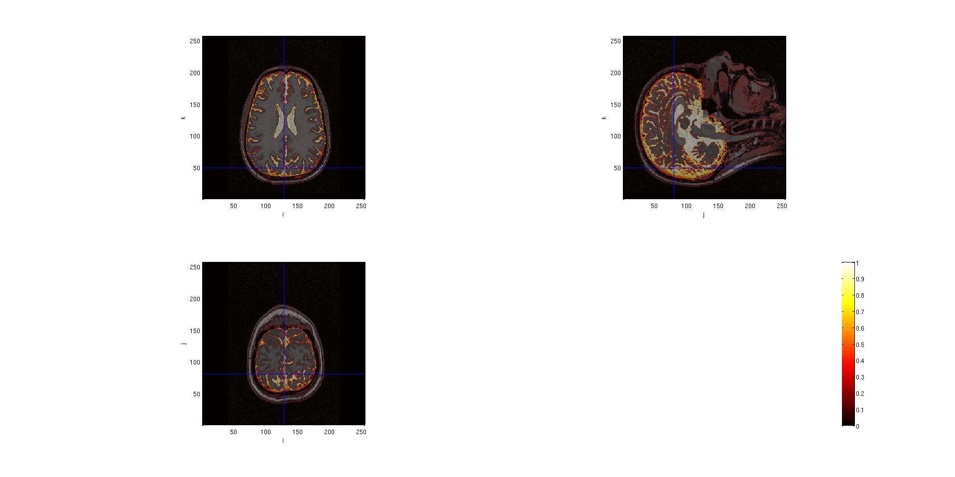
Here are the outputs of ft_volumesegment on data from a .mgz volume, plotted with ft_sourceplot.
seg.gray

seg.white
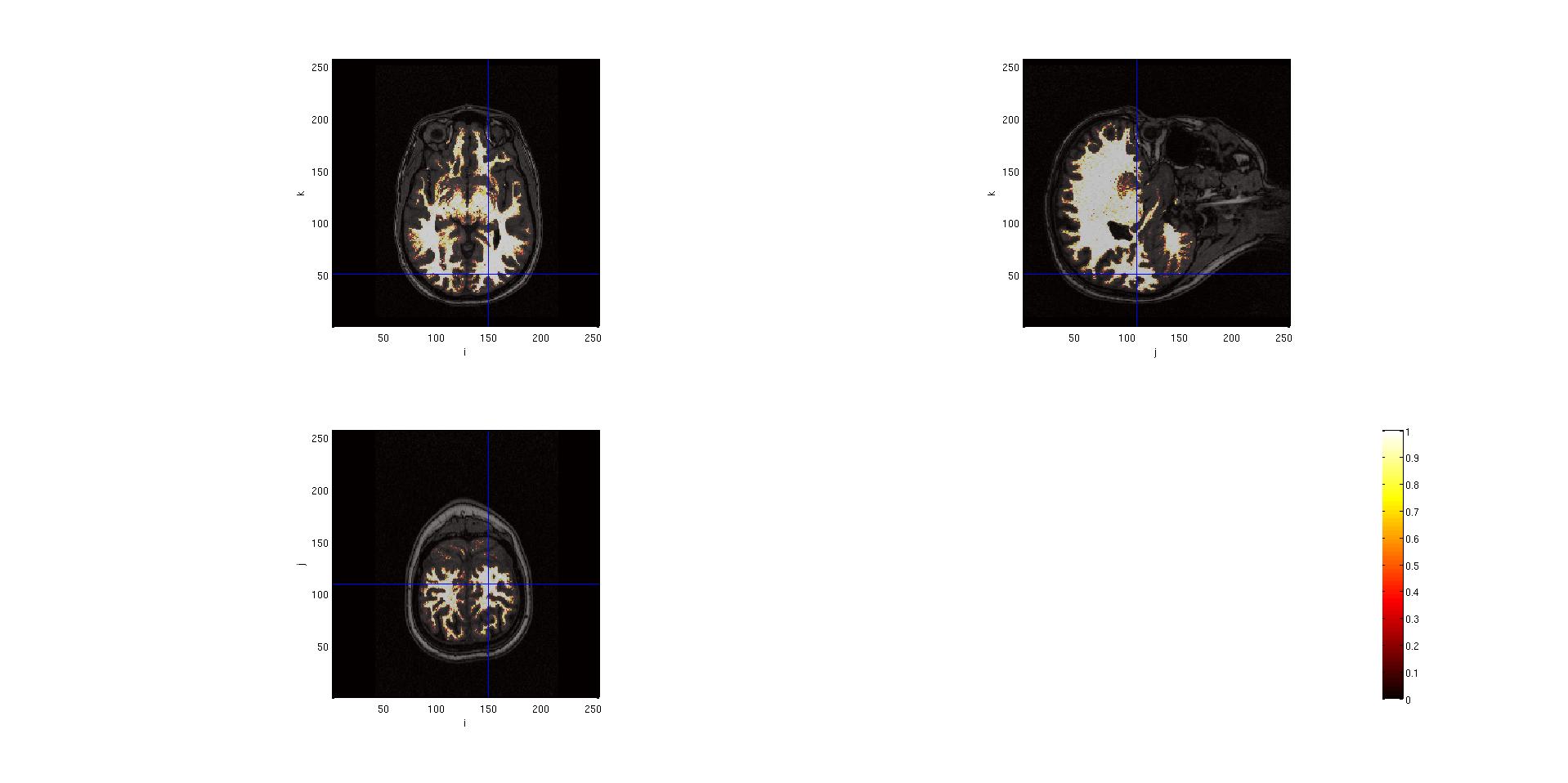
seg.csf
This segmentation is not the same what MNE does with the help of FS. In order to make BEM meshes, one should create a volume that contains the brain, the brain with (or until) the skull and the entire head until the skin. For creating BEM meshes, I have followed the “Create BEM headmodel for EEG” example script. This script needs a proper documentation because it is difficult to figure out to what one should attend during creating the brain, skin, skull volumes.
There are no FT functions for creating meshes, but the MATLAB image processing toolbox is used. It takes time to create the meshes.
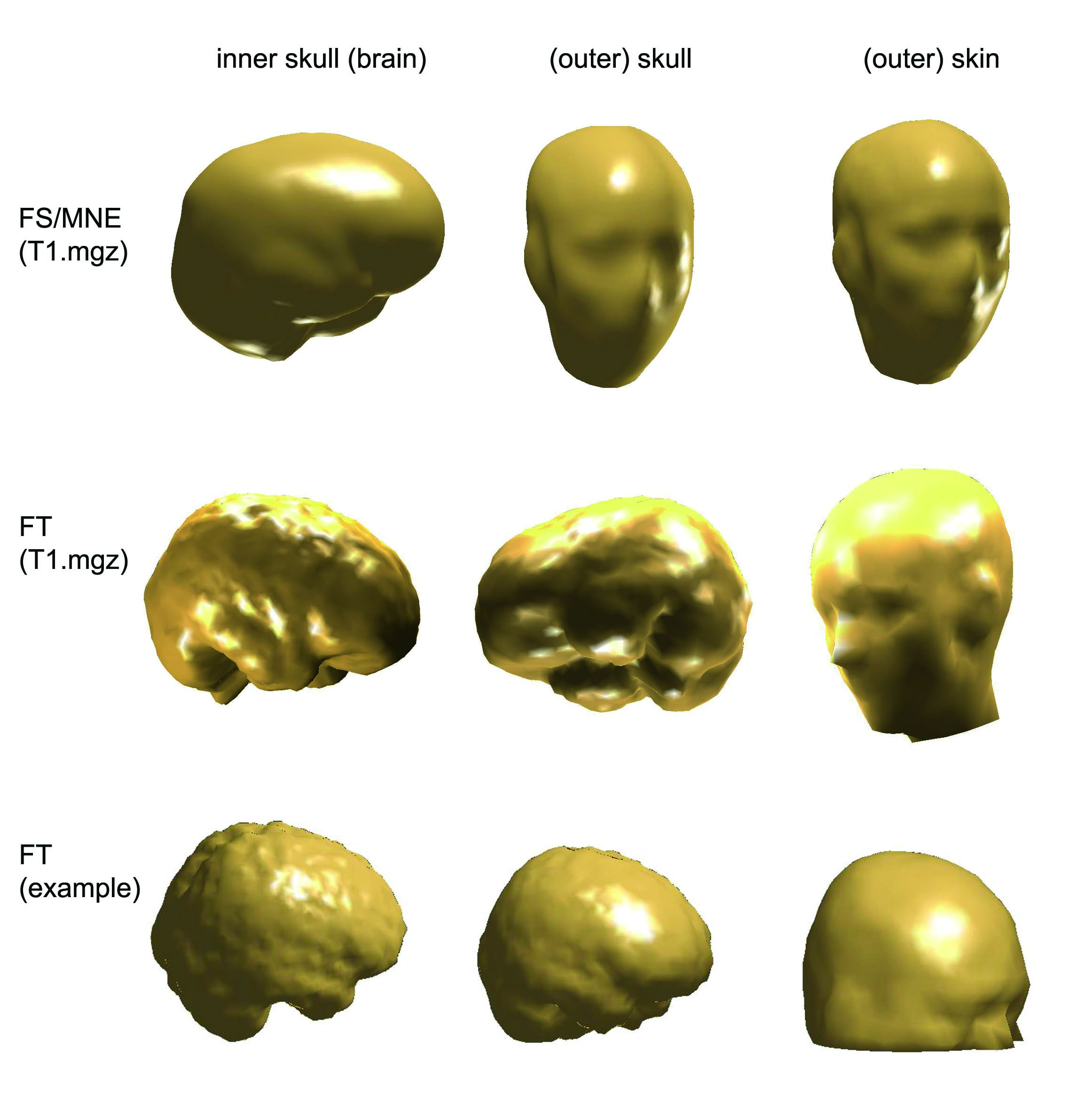
Comparing BEM meshes
I have created BEM meshes in three way
- I have the BEM meshes created by FreeSurfer
- I have created BEM meshes with FieldTrip, using the same T1.mgz volume that FS used for creating meshes. (It is a conformed (256x256x256) volume with intensity normalization.)
- I have created BEM meshes with FieldTrip, using a .mnc volume (downloaded from internet). This sort of volume was used also in the tutorial example script of FieldTrip.
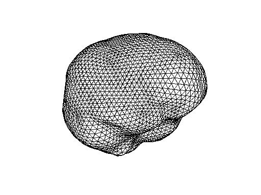
I could read in the FS/MNE BEM meshes in F
innerskull = ft_read_headshape('$SUBJECTS_DIR/<subject's name>/bem/<subject's name>-inner_skull-5120.surf');
This is the code for plotting a mesh that was created by FS/MN
ft_plot_mesh(innerskull,'facecolor','skin');camlight;
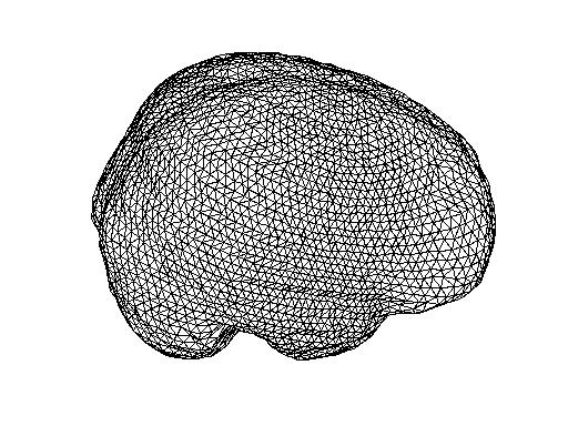
And this is for plotting a mesh (inner skull) created by F
ft_plot_mesh(vol.bnd(3),'facecolor','skin');camlight;
The following picture show the BEM meshes
Preprocessing MEG data
Preprocessing
For more information in how to read in MEG data into MATLAB, how to segment the data and how to do artifact-rejection see the other tutorials.
:!: One big difference between FT and MNE is that MNE is doing only automatic artifact-rejection.
Averaging and noise-covariance estimation
Both calculation can be done with ft_timelockanalysis function on the preprocessed, segmented and artifact-free data.
cfg  = [];
cfg.channel = 'MEG';
tlck = ft_timelockanalysis(cfg, data);

cfg         = [];
cfg.latency = [-inf 0];
cfg.keeptrials = 'yes';
cfg.covariance = 'yes';
cfg.channel = 'MEG';
cfg.covariancewindow = cfg.latency;
tlckb       = ft_timelockanalysis(cfg, data);
:?: It is not clear for me yet, what is (or should be) the covariance window.
In MNE, it is possible (and recommended) to remove a baseline from the epochs before they are included in the noise-covariance estimation.
Forward solution
This code shows how to calculate the forward solution in FieldTrip. It needs the volume conductor model (vol), the source space (bnd3) and position of the gradiometers that contained in the data structure (data.grad).
First, the units of the source space should be converted because all units should be in ‘cm’.
bnd3.unit = 'mm';
bnd3 = ft_convert_units(bnd3, 'cm');


cfg = [];
cfg.grad = data.grad;
cfg.headmodel = vol;
cfg.sourcemodel.pos = bnd3.pnt;
cfg.sourcemodel.inside = 1:size(bnd3.pnt,1);
cfg.channel = 'MEG';
grid = ft_prepare_leadfield(cfg);
Inverse solution
This code shows how to calculate the inverse solution in FieldTrip. It needs the volume conductor model (vol), the leadfield (grid), the noise-covariance estimation (that is an average of the covariances), the source-covariance (that is an identity matrix here) and the data.
cfg = [];
cfg.method = 'mne';
cfg.grid = grid;
cfg.headmodel = vol;
cfg.mne.noisecov = squeeze(mean(tlckb.cov));
cfg.mne.sourcecov = speye(numel(grid.leadfield)*3);
cfg.mne.lambda  = 1e13;
source = ft_sourceanalysis(cfg, tlck);
Visualization
Step 2: Testing the equality of FT vs. MNE Suite
Testing the minimum-norm estimate
Testing minimum-norm estimate in FieldTrip and in MNE Suite
Test on phantom data
| Phantom data | MNE Suite | FieldTrip | FieldTrip |
|---|---|---|---|
| Plot inverse solution at max (in time) | [1] | [2]] | [3] |
| leadfield | mne | fieldtrip | mne |
| volume conductor | icosahedron642 | single sphere | single sphere |
| source space | grid with 635 points | grid with 641 points | grid with 635 points |
| lambda | 0.01 | ||
| noise-covariance matrix | eye(186) | eye(151) | |
| source-covariance | ? no depth weighting | depth weighting |
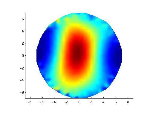
Plot inverse solution at max (in time):
[1]
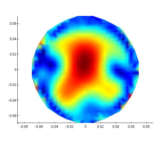
[2]

[3]
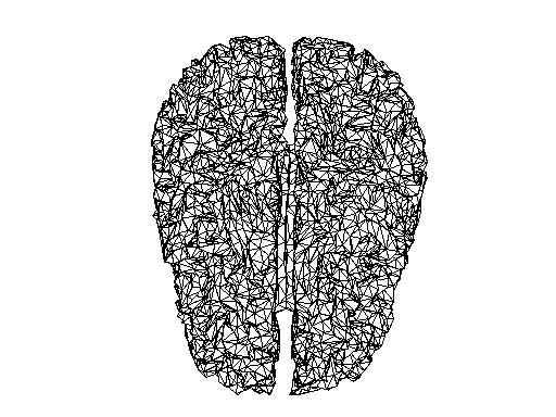
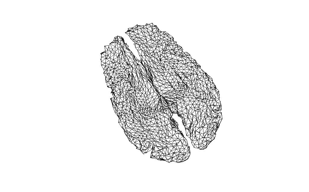
Comparing source spaces
I have read in the source space created on the sample data (subject 10 in Lin’s experiment) into MATLAB.
In MNE:
mne_setup_source_space --ico -6
In MATLAB:
src = mne_read_source_spaces('/<path>/sub10-oct-6-src.fif');

bnd_mne = [];
bnd_mne.pnt=[src(1).rr; src(2).rr];
bnd_mne.tri=[src(1).use_tris; src(2).use_tris + size(src(1).rr,1)];

figure;
ft_plot_mesh(bnd_mne)
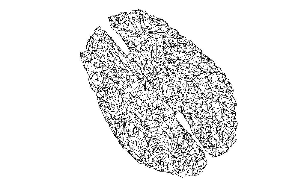
And the source space of the same volume created in FieldTrip, and reduced to the same number of vertices with the MATLAB reducepatch function
bnd2_ft = bnd_ft;
[bnd2_ft.tri, bnd2_ft.pnt]=reducepatch(bnd_ft.tri, bnd_ft.pnt, 16384);

ft_plot_mesh(bnd2_ft);
Step 3: Tutorial
Source reconstruction of event-related fields using minimum-norm estimate
References
Matti Hämäläinen, MNE software User’s Guide. Version 2.7
FreeSurfer Wiki, http://surfer.nmr.mgh.harvard.edu/fswiki