Localizing the sources underlying the difference in event-related fields

Background

Activity of neuronal sources can be measured with EEG or MEG as event-related potentials or fields. A general principle for EEG and MEG source analysis is that of superposition. The channel-level spatial distribution of the activity of one source and that of another source will be different. That difference is easy to recognize if one source is active in one experimental condition and the other source in another condition. The superposition principle states that if two sources are simultaneously active, the resulting channel-level spatial distribution is equal to the sum of the channel-level spatial distribution of the two sources separately.

Reconstructing the source location in case of simultaneous activity of multiple sources is more difficult than localizing a single source. However, the superposition principle can effectively be used in source lozalization if two experimental conditions differentiate the strenth of the two sources.

Consider a source in area A1 with a channel-level spatial field distribution F1 of and another source in area A2 with field distribution F2. If the source 1 is active with strength one and source 2 with strength zero, the field distribution can be described as “one times F1”. If both sources are active, the field distribution is “one times F1 plus one times F2”. In general the field distribution of source 1 with strength S1 and source 2 with strength S2 is

F(combined)  = S1 * F1  + S2 * F2

If the source strength S1 and/or S2 can be differentiated by an experimental manipulation, the respective contributions to the combined field distributions will differ. For example

F(condA) = 1.0 * F1 + 0.3 * F2

and

F(condB) = 1.0 * F1 + 0.2 * F2

In this example the activity of source 1 is not different in the two conditions, but the strength of source 2 is slightly weaker in the second condition.

In either condition A or condition B, the field distribution is dominated by source 1 and it will not be apparent that multiple dipoles are required for a correct source reconstruction of either condition. After a dipole fit of either condition with a single dipole the goodness of fit (or residual variance) will also not give a clear indication that the model is inappropriate. Attempting a source reconstruction of the field distribution produced by two sources in general will result in a dipole with a location representing the center of mass of the activity of the two actual sources. If the sources are equally strong, this will result in the dipole in between the two actual sources.

Dipole fitting works by minimizing the error between the model and measured data. In this example the stronger source 1 has much more contribution to this error, and hence on the resulting dipole location. Therefore if one source is stronger than the other, the center of mass and the fitted dipole will be closer to that stronger source. In the example above, source 1 is considerably stronger than source 2 in both conditions. The resulting dipole location for condition A and B therefore will be very similar, with only a small shift of the center of mass (dipole location) towards S1 in condition B. Since there is also noise in the data, there will be some added random fluctuation in the dipole location in both conditions, making it even more difficult to distinguish and interpret the underlying source differences.

Now consider computing the difference event-related field as

F(diff) = F(condA) - F(condB)
F(diff) = (1.0 * F1 + 0.3 * F2) - (1.0 * F1 + 0.2 * F2)
F(diff) = 1.0 * F1 - 1.0 * F1 + 0.3 * F2 - 0.2 * F2
F(diff) = 0.1 * F2

i.e. the difference field reflects only the weak difference of source 2, and the equal-strength contribution of source 1 is completely gone in the difference field. A source reconstruction of the resulting field distribution will result in a dipole at the location of source 2.

To summarise, the source reconstruction of combined activity with a single-dipole model results in the dipole reflecting the center of mass of the activity. If the activity of a single contributing source can be experimentally manipulated, the source reconstruction of the difference field will result in a dipole at the exact location of that differentially strong source.

In reality, it is more likely that the experimental manipulation will not only affect the strength of one source, but rather that of both sources. Even in that case looking at the distribution of the difference field is instructive. For example, if F(condA) = 1.0 * F1 + 0.3 * F2 and F(condB) = 0.9 * F1 + 0.2 * F2 then F(diff) = 0.1 * F1 + 0.1 * F2

Here the original field distributions in both conditions are dominated by the strongest source 1, whereas the difference field reveals source 1 and 2 equally strong. Source reconstruction of the difference field in this case would involves a fit with a two-dipole model. Important is that just by eye-balling the spatial distribution it is already possible to distinguish the two sources, whereas the original field distributions of the two original conditions will be difficult, if not impossible, to distinguish.

Applied to the experimental data

In this experiment, MEG was recorded during stimulation of the affected/painful hand prior to, and after application of a pain blocker. These correspond to the conditions A and B as explained above. First the MEG topography of the M24 event-related field is given for both conditions separately.

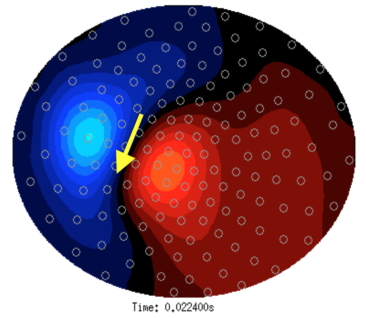
Figure: A16/SV-med-R (i.e. pain)

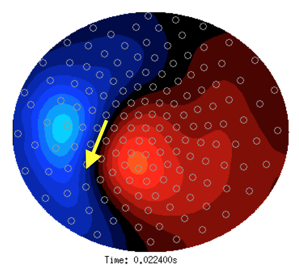
Figure: A16/SV-med-R-block (i.e. no pain)

Looking at these two topographies, a single dipole seems sufficient to explain the field distribution. It is also not clear that the dipole would be at a different location, although there is a small change in the global field strength. A dipole that corresponds with the dipolar field is schematically drawn in the two topographies as a yellow arrow. Subsequently we can look at the difference map (see below).

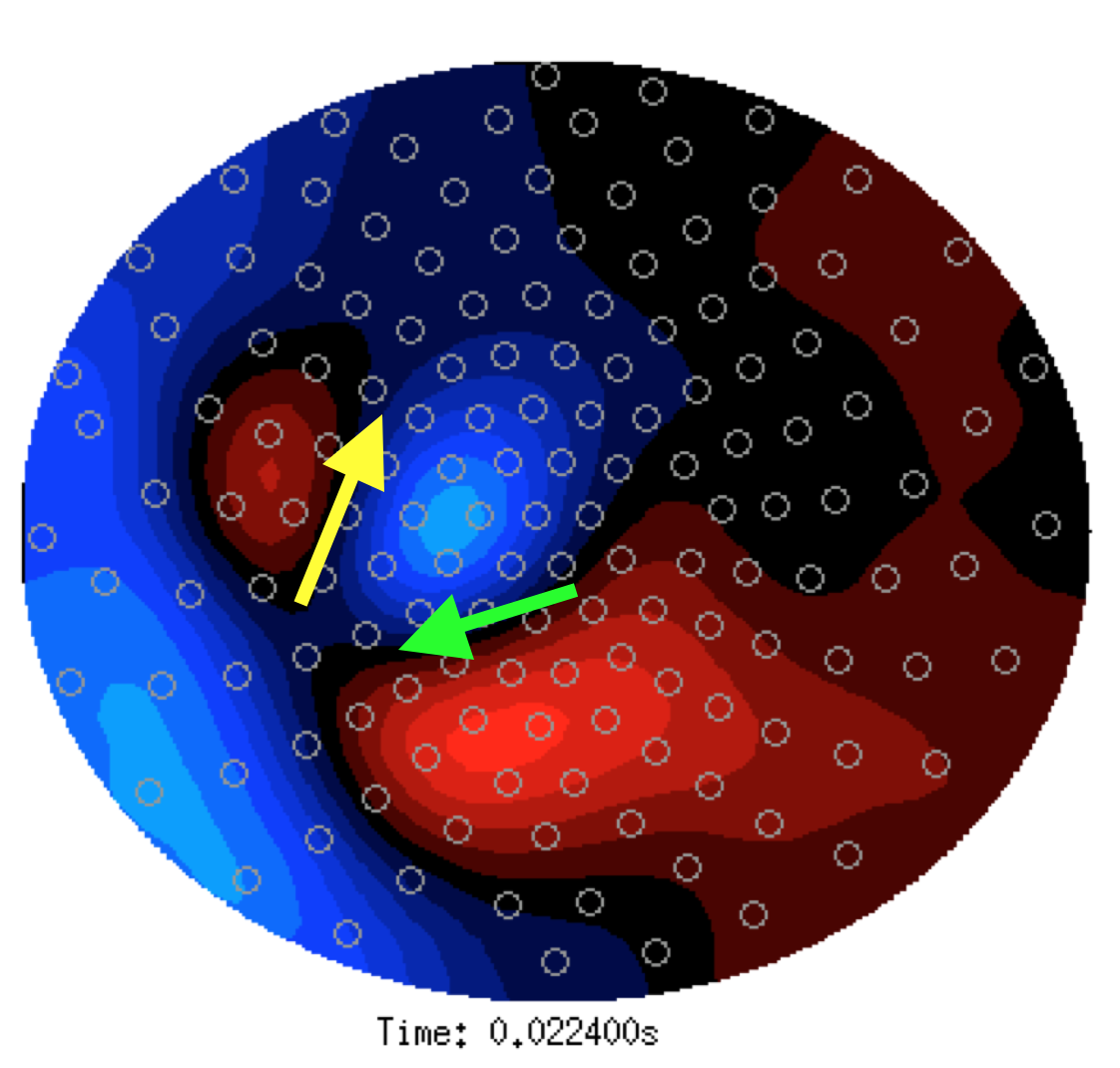
Figure: difference = block - pain

The difference map shows two dipolar patterns with opposing directions. The negativity (ingoing field) of the two dipolar fields is approximately at the same sensor location. The first dipolar field resembles the distribution in the two separate conditions above. In the difference topography that is (again) schematically indicated with a yellow arrow. The source corresponding with the yellow arrow has a smaller amplitude in the block condition than in the pain condition, which can be derived from the opposite direction of the arrow (note the subtraction is block-pain).

A second dipolar field that is more posterior and slightly more central is now also visible (indicated with a green arrow). This green source is not obvious in either separate condition.

Given the two source locations that can be identified from the difference map, it makes sense to estimate the source strength for each of the two sources in both separate conditions (i.e. fit the strength, not the location), and explicitly compare the dipole strength between the two conditions for each dipole. It might be possible to get a better estimate of the source location by performing a dipole fit with two dipoles on the grand average of the two conditions, as that results in a better signal to noise, and under the null-hypothesis the sources are the same anyway. The optimal source locations can then be fixed and source strength can again be estimated for each separate condition and compared over conditions.

To summarize, using the “difference dipole fit “ approach reveals two sources that contribute to the M24 event-related field, and differentiates the effect of the application of a pain blocker onto the two sources.

Doing this in FieldTrip

To compute the difference ERF or ERP in FieldTrip, you would use ft_timelockanalysis on each of the conditions, followed by ft_math to compute the difference. The difference is used in ft_dipolefitting or ft_sourceanalysis.