Analyzing NIRS data recorded during unilateral finger- and foot-tapping
This example script demonstrates the analysis of data that is shared by Sujin Bak, Jinwoo Park, Jaeyoung Shin, and Jichai Jeong: Open Access fNIRS Dataset for Classification of Unilateral Finger- and Foot-Tapping.
The following links point to the shared data, to the PDF manuscript that explains the shared data, and to a GitHub repository from one of the authors that contains some example analyses on the data.
- https://doi.org/10.6084/m9.figshare.9783755.v2
- https://doi.org/10.3390/electronics8121486
- https://github.com/JaeyoungShin/fNIRS-dataset
The data includes the concentration changes of oxygenated/reduced hemoglobin ∆HbO/HbR, trigger information, and fNIRS channel information. The recordings were done for 30 subjects that were performing a finger- and foot-tapping task.
The data were recorded by a three-wavelength continuous-time multi-channel fNIRS system (LIGHTNIRS, Shimadzu, Kyoto, Japan) consisting of eight light sources (Tx) and eight detectors (Rx). Four each of Tx and Rx were placed around C3 on the left hemisphere, and the rest were placed around C4 on the right hemisphere.
The temporal structure of each trial is
- instruction for 2s
- fixation cross, this indicates that the task has to be executed, for 10s
- “stop” for 2s
- fixation cross indicating rest period, for 15-17 seconds
The total duration of a trial, including the instruction, ranges from 2+10+2+15=29 to 2+10+2+17=31 seconds.
Building a MATLAB analysis script
filenames = {
  'v2/fNIRS 01.mat'
  'v2/fNIRS 02.mat'
  'v2/fNIRS 03.mat'
  'v2/fNIRS 04.mat'
  'v2/fNIRS 05.mat'
  'v2/fNIRS 06.mat'
  'v2/fNIRS 07.mat'
  'v2/fNIRS 08.mat'
  'v2/fNIRS 09.mat'
  'v2/fNIRS 10.mat'
  'v2/fNIRS 11.mat'
  'v2/fNIRS 12.mat'
  'v2/fNIRS 13.mat'
  'v2/fNIRS 14.mat'
  'v2/fNIRS 15.mat'
  'v2/fNIRS 16.mat'
  'v2/fNIRS 17.mat'
  'v2/fNIRS 18.mat'
  'v2/fNIRS 19.mat'
  'v2/fNIRS 20.mat'
  'v2/fNIRS 21.mat'
  'v2/fNIRS 22.mat'
  'v2/fNIRS 23.mat'
  'v2/fNIRS 24.mat'
  'v2/fNIRS 25.mat'
  'v2/fNIRS 26.mat'
  'v2/fNIRS 27.mat'
  'v2/fNIRS 28.mat'
  'v2/fNIRS 29.mat'
  'v2/fNIRS 30.mat'
  };

% this allows switching easily between subjects, and eventually looping over all 30 subjects
filename = filenames{1};
Exploring the MATLAB files that hold the NIRS data
The data is shared by the authors in the form of MATLAB files. Each file contains a bunch of separate variables, you can load it like this to represent it as a structure:
nirs = load(filename);

>> nirs
nirs =
  struct with fields:
     mrk: [1x1 struct]
     mnt: [1x1 struct]
     nfo: [1x1 struct]
     ch1: [30003x1 double]
     ch2: [30003x1 double]
     ch3: [30003x1 double]
     ch4: [30003x1 double]
     ch5: [30003x1 double]
     ch6: [30003x1 double]
     ch7: [30003x1 double]
     ch8: [30003x1 double]
     ch9: [30003x1 double]
    ch10: [30003x1 double]
    ch11: [30003x1 double]
    ch12: [30003x1 double]
    ch13: [30003x1 double]
    ch14: [30003x1 double]
    ch15: [30003x1 double]
    ch16: [30003x1 double]
    ch17: [30003x1 double]
    ch18: [30003x1 double]
    ch19: [30003x1 double]
    ch20: [30003x1 double]
    ch21: [30003x1 double]
    ch22: [30003x1 double]
    ch23: [30003x1 double]
    ch24: [30003x1 double]
    ch25: [30003x1 double]
    ch26: [30003x1 double]
    ch27: [30003x1 double]
    ch28: [30003x1 double]
    ch29: [30003x1 double]
    ch30: [30003x1 double]
    ch31: [30003x1 double]
    ch32: [30003x1 double]
    ch33: [30003x1 double]
    ch34: [30003x1 double]
    ch35: [30003x1 double]
    ch36: [30003x1 double]
    ch37: [30003x1 double]
    ch38: [30003x1 double]
    ch39: [30003x1 double]
    ch40: [30003x1 double]
     dat: [1x1 struct]
Contrary to the description in the accompanying publication (see table 1 in the PDF manuscript) and in the GitHub repository, the MATLAB files do not contain the variables cntHb, clab, etc. However, it is not so hard to make sense of the data: each channel is represented as a vector, there is header information, there is information about the optode montage, and there is information about the events.
>> nirs.nfo
ans =
  struct with fields:
            fs: 13.3333
          clab: {1x40 cell}
             T: 30003
       nEpochs: 1
        length: 2.2502e+03
        format: 'DOUBLE'
    resolution: [1x40 double]
          file: 'D:\Experimental data\NIRS motor imagery\matdata\fNIRS 01'
       nEvents: 75
      nClasses: 3
     className: {'RIGHT'  'LEFT'  'FOOT'}


>> nirs.mnt
ans =
 struct with fields:
              x: [40x1 double]
              y: [40x1 double]
         pos_3d: [3x40 double]
           clab: {1x40 cell}
            box: [2x41 double]
         box_sz: [2x41 double]
      scale_box: [2x1 double]
   scale_box_sz: [2x1 double]


>> nirs.mrk
ans =
 struct with fields:
       event: [1x1 struct]
        time: [1x75 double]
           y: [3x75 double]
   className: {'RIGHT'  'LEFT'  'FOOT'}
Converting the MATLAB structure to a FieldTrip raw data structure
Since the data is not stored on disk in a dataformat that FieldTrip can directly read, we will circumvent the FieldTrip reading functions as outlined in this frequently asked question.
We start with constructing a MATLAB data structure according to ft_datatype_raw, as if it were produced by ft_preprocessing.
data_raw = [];
data_raw.label = nirs.nfo.clab(:);
data_raw.trial{1} = [
  % transpose each channel, we want the data matrix to be Nchans * Nsamples
  nirs.ch1'
  nirs.ch2'
  nirs.ch3'
  nirs.ch4'
  nirs.ch5'
  nirs.ch6'
  nirs.ch7'
  nirs.ch8'
  nirs.ch9'
  nirs.ch10'
  nirs.ch11'
  nirs.ch12'
  nirs.ch13'
  nirs.ch14'
  nirs.ch15'
  nirs.ch16'
  nirs.ch17'
  nirs.ch18'
  nirs.ch19'
  nirs.ch20'
  nirs.ch21'
  nirs.ch22'
  nirs.ch23'
  nirs.ch24'
  nirs.ch25'
  nirs.ch26'
  nirs.ch27'
  nirs.ch28'
  nirs.ch29'
  nirs.ch30'
  nirs.ch31'
  nirs.ch32'
  nirs.ch33'
  nirs.ch34'
  nirs.ch35'
  nirs.ch36'
  nirs.ch37'
  nirs.ch38'
  nirs.ch39'
  nirs.ch40'
  ];
data_raw.fsample = nirs.nfo.fs;
data_raw.time{1} = ((1:nirs.nfo.T)-1)/nirs.nfo.fs;
Convert the optode montage to a layout for plotting
In FieldTrip we can have a detailed description of the NIRS optode placement and how optodes are combined to form channels. However, in this dataset this information is not complete and we cannot make a complete opto structure.
This is how far we can get
opto = [];
opto.label = nirs.mnt.clab(:);
opto.chanpos = nirs.mnt.pos_3d'; % these are all nan
But this is not a complete description of the channel and sensor information according to ft_dataype_sens. However, a full sensor definition is also not required: the optical densities have already been converted in HbO and HbR prior to sharing, so we only care about channel positions for plotting.
For the plotting of channel level data (see also this tutorial) we need a 2D layout. That is explained in detail in this tutorial. If the opto definition had included 2D or 3D channel positions, then we could have used ft_prepare_layout but now we will manually construct the layout structure.
layout = [];
layout.label = nirs.mnt.clab(:);
layout.pos = [nirs.mnt.x(:) nirs.mnt.y(:)]; % these are all nan
layout.pos = nirs.mnt.box';
layout.width = nirs.mnt.box_sz(1,:)';
layout.height = nirs.mnt.box_sz(2,:)';
layout.outline = {};
layout.mask = {};
I don’t think that the 41st position refers to an actual channel, so let’s remove that.
layout.pos(41, :) = [];
layout.width(41)  = [];
layout.height(41) = [];
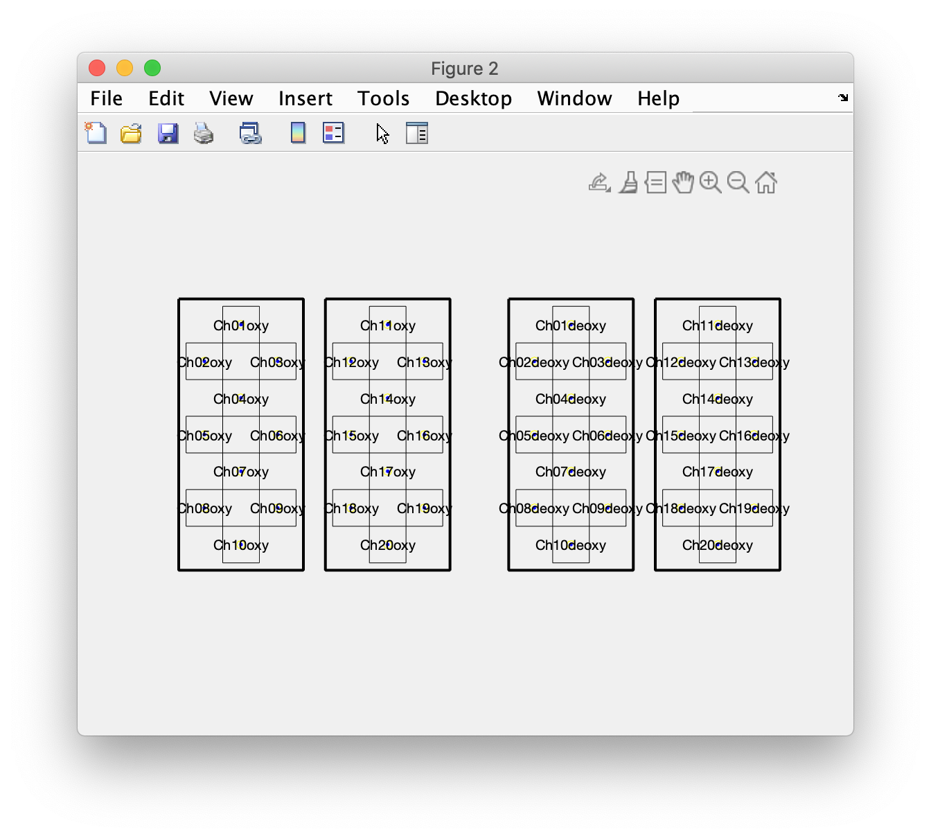
We can plot the layout using ft_plot_layout and inspect it in detail. That is something I have done multiple times, going back and forth in the script to ensure that my interpretation of the mnt field matches the data.
figure
ft_plot_layout(layout, 'label', true)

This shows four groups, with two groups of oxy channels on the left of the figure (for the left and right hemisphere), and the corresponding deoxy channels on the right of the figure. This matches with the schematic display in figure 1 of the PDF manuscript, and with the displayed data in figure 3 of the PDF manuscript.
To improve the plotting of topographies, we can also make an outline and mask. The outline comproses extra lines that are added to the figure, often we include a circle (representing the head) with a triangle at the top (representing the nose). The mask comprises a series of polygons that are used in topographic interpolation and masking the interpolated data that is outside the head, but also by masking the interpolated data that is in between the grid on the left and right hemisphere. This will become more clear at the end of this example script.
pad = 0.2;
section = {1:10 11:20 21:30 31:40};
for i=1:4
  sel = section{i};
  % upper left
  corner1x = min(layout.pos(sel,1)-layout.width (sel)/2) - pad;
  corner1y = max(layout.pos(sel,2)+layout.height(sel)/2) + pad;

  % upper right
  corner2x = max(layout.pos(sel,1)+layout.width (sel)/2) + pad;
  corner2y = max(layout.pos(sel,2)+layout.height(sel)/2) + pad;

  % lower right
  corner3x = max(layout.pos(sel,1)+layout.width (sel)/2) + pad;
  corner3y = min(layout.pos(sel,2)-layout.height(sel)/2) - pad;

  % lower left
  corner4x = min(layout.pos(sel,1)-layout.width (sel)/2) - pad;
  corner4y = min(layout.pos(sel,2)-layout.height(sel)/2) - pad;

  layout.outline{i} = [
    corner1x corner1y
    corner2x corner2y
    corner3x corner3y
    corner4x corner4y
    corner1x corner1y % this closes the outline
    ];

  layout.mask{i} = [
    corner1x corner1y
    corner2x corner2y
    corner3x corner3y
    corner4x corner4y
    corner1x corner1y % this closes the outline
    ];
end

figure
ft_plot_layout(layout, 'label', true, 'outline', true, 'mask', true)
The layout now also shows the outline, as thick black lines. If you disable the outline, you can also see the mask as dotted lines.
Parsing the events and segmenting the data in trials
In general in FieldTrip events have to be aligned with samples. The first sample of a recording on disk is referred to as sample 1.
The mrk field contains times
>> nirs.mrk.time
ans =
  Columns 1 through 9
        1950    30975    60975    91950    ...
These numbers are larger than the total number of samples, so they do not directly map onto samples. I started off assuming that the marker time is expressed in milliseconds, but that turned out not to be correct. Therefore I experimented with the following piece of code until I had something that made sense.
This timestamp to sample ratio results in the events being nicely spaced over the whole experiment
ratio = 75;
Note that 1/data.fsample = 0.075, i.e., with the 13.333 Hz sampling rate each sample happens to be 75 ms. When working with unknown data it is not uncommon to have to deal with a puzzle like this, it reminds me of Kabbalah.
event = [];
for i=1:nirs.nfo.nEvents
event(i).type = 'marker';
event(i).value = nirs.mrk.className{nirs.mrk.event.desc(i)};
event(i).sample = round(nirs.mrk.time(i)/ratio) + 1;
event(i).duration = nan;
event(i).offset = nan;
end
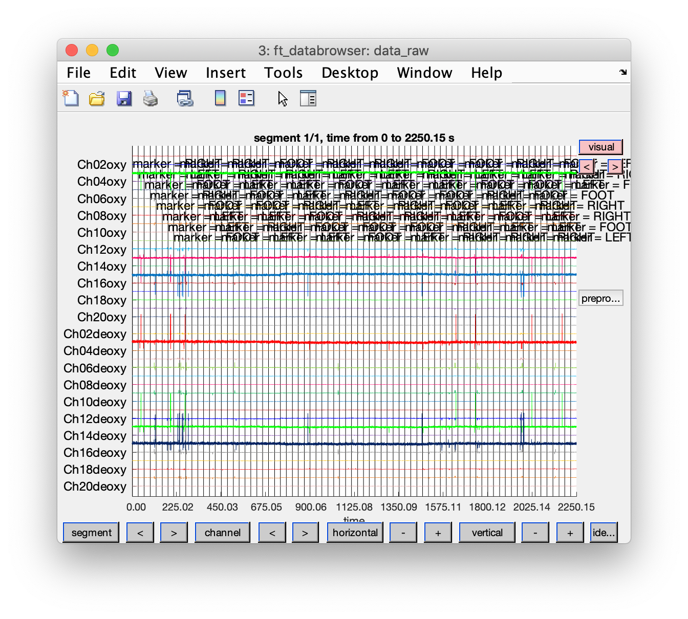
cfg = [];
cfg.event = event; % store the events in the configuration to have them displayed
cfg.viewmode = 'vertical';
cfg.preproc.demean = 'yes';
cfg.blocksize = nirs.nfo.length; % show the data over the whole length
ft_databrowser(cfg, data_raw);
Apply a band-pass filter on the continuous data
cfg = [];
cfg.bpfilter = 'yes';
cfg.bpfreq = [0.02 0.8];
cfg.bpfilford = 2;
data_filt = ft_preprocessing(cfg, data_raw);
Segment the continuous data into trials
To segment the data we have to create a so-called “trial definition”. This would normally be done using ft_definetrial and using the events that were read from the data on disk (had it been a supported file format). The trial definition specifies the begin and end sample of each trial, and the offset, i.e., how many samples the time defined as t=0 is shifted relative to the data segment. Furthermore, it can contain additional columns with trial specific information, such as condition codes.
The temporal structure of each trial is
- instruction for 2s
- fixation cross, this indicates that the task has to be executed, for 10s
- “stop” for 2s
- fixation cross indicating rest period, for 15-17 seconds
The total duration of a trial, including the instruction, ranges from 2+10+2+15=29 to 2+10+2+17=31 seconds.
We will use the standard FieldTrip event structure to make the trials, this is also what ft_read_event returns for supported data formats.
taskonset = [event.sample];  % let's assume that the marker is at task onset
begsample = taskonset - 2*data_raw.fsample;
endsample = taskonset + (10+2+15)*data_raw.fsample;
offset = - 2*data_raw.fsample * ones(size(begsample)); % each trial has the same 2 seconds offset
The begin sample, end sample and offset should be integers:
begsample = round(begsample);
endsample = round(endsample);
offset = round(offset);
and we map the right, left, and foot condition onto condition codes 1, 2, and 3.
[dummy, condition] = ismember({event.value}, {'RIGHT'  'LEFT'  'FOOT'});

trl = [begsample(:) endsample(:) offset(:) condition(:)];

cfg = [];
cfg.trl = trl;
data_segmented = ft_redefinetrial(cfg, data_filt);
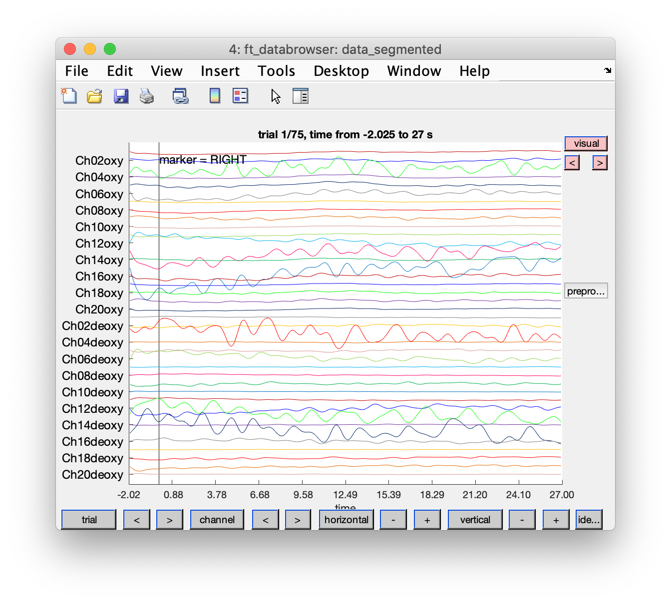
Visualize the segmented data
cfg = [];
cfg.event = event;
cfg.viewmode = 'vertical';
cfg.preproc.demean = 'no'; % it is filtered by now
ft_databrowser(cfg, data_segmented);
Average the segmented data, conditional on each condition
cfg = [];
cfg.trials = data_segmented.trialinfo==1;
timelockRight = ft_timelockanalysis(cfg, data_segmented);
cfg.trials = data_segmented.trialinfo==2;
timelockLeft = ft_timelockanalysis(cfg, data_segmented);
cfg.trials = data_segmented.trialinfo==3;
timelockFoot = ft_timelockanalysis(cfg, data_segmented);
Plot the averaged responses
Running this script for some of the subjects, I noticed that the the data of subject 1 is very nice, even without artifact removal. The data of subjects 2 and 3 is not so nice their results would probably improve by including some additional cleaning and artifact removal in the script.
cfg = [];
cfg.layout = layout;
cfg.showoutline = 'yes';
cfg.baseline = [-2 0];
cfg.showlabels = 'yes';
cfg.interactive = 'no'; % use MATLAB for zooming in
ft_multiplotER(cfg, timelockRight, timelockLeft, timelockFoot);
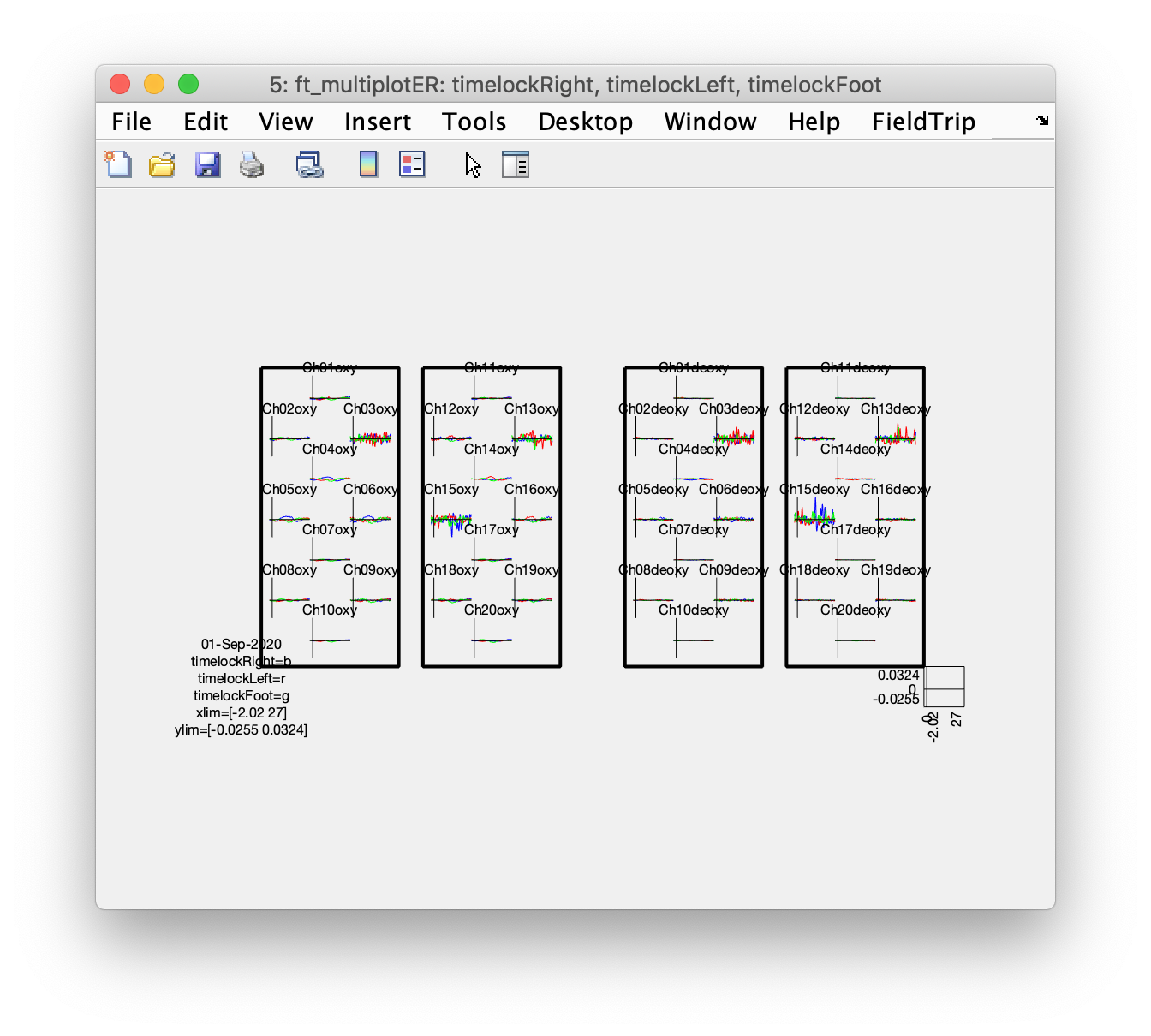
Although some of the more noisy channels dominate the figure due to the automatic vertical scaling, if you zoom in and pay attention to Ch4oxy, Ch5oxy, and Ch6oxy over the left hemisphere, and Ch14oxy and Ch16oxy over the right hemisphere, you can see that the left hemisphere shows more activity during the right fingertapping task (blue) and the right hemisphere shows more activity following the left fingertapping task (red).
This example script explains in more detail how for a NIRS dataset the oxy and deoxy channels can either be plotted on top of each other (which is spatially consistent with how the data is recorded) or side-by-side. Plotting them side-by-side makes the results easier to interpret, especially if you have multiple responses (like we have here for left, right and foot conditions). For plotting topographic distributions you also have to ensure that your 2D channel layout does not have overlapping channels that have bvery different numbers.
Plot the topography of the averaged responses
This step benefits from the layout having an outline and especially a mask, otherwise the interpolation will cause the whole image to be color coded, including the pieces in between the hemispheres and in between the oxy (on the left) and deoxy channels (on the right).
cfg = [];
cfg.layout = layout;
cfg.interactive = 'yes';
cfg.xlim = [7 15];
cfg.ylim = [-0.004 0.004];
figure; ft_topoplotER(cfg, timelockRight);
figure; ft_topoplotER(cfg, timelockLeft);
figure; ft_topoplotER(cfg, timelockFoot);

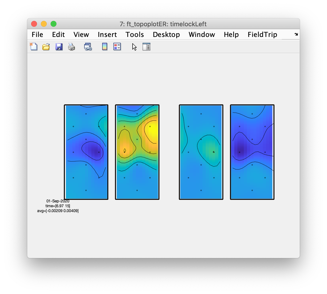
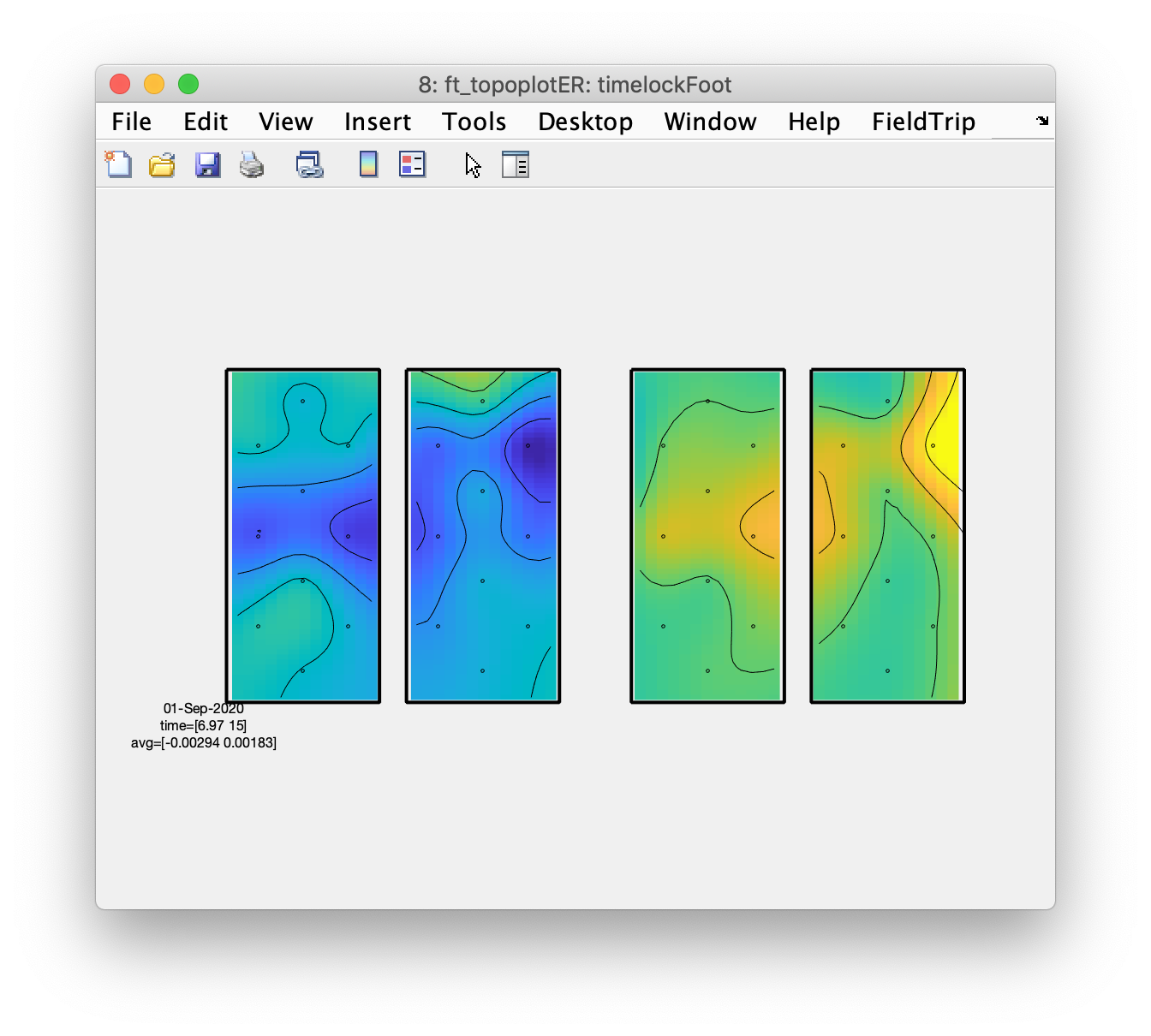
From the topographic arrangements it is clear that the left hemisphere responds with an increase in HbO to the right fingertapping task and the right hemisphere to the left fingertapping task; the HbR (on the right side of the figure) shows the opposite pattern. Also interesting is that both left and right hemisphere show a decrease in HbO and an increase in HbR during the tapping of the foot.