Tags: example statistics

Stratify the distribution of one variable that differs in two conditions

This example script demonstrates two stratification methods. In the first, the extremes are trimmed, such that at the end the mean of the distributions is (close to) equal. In the second the distribution itself is equated, including the mean, variance and all higher order statistics. Note that, although the second method looks nicer, it is not completely flawless. There is still a small bias within each bin for the selected items to be shifted, and hence the two distributions will not be perfectly equal.

Finally, this example page shows how you can very simply stratify with the FieldTrip ft_stratify function. Although the example here only looks at a single channel, quite often you’ll want to stratify the power in two channels simultaneously (e.g., for coherence computation). The ft_stratify function allows you to do that, and also solves the within-bin bias problem (cfg.equalbinavg=’yes’).

s1_orig = randn(1,10000);
s2_orig = randn(1,10000) + 1;

%%%%%%%%%%%%%%%%%%%%%%%%%%%%%%%%%%%%%%%%%%%%%%%%%%%%%%%%%%%%%%%%%%%%%%%%

s1 = s1_orig;
s2 = s2_orig;

s = [s1(:) s2(:)];
figure; hist(s, 100)

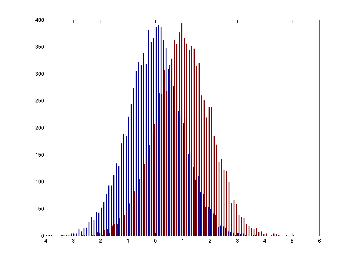
Figure 1: Two distributions with different means.

% trim the extremes
s1 = sort(s1);
s2 = sort(s2);

m1 = mean(s1);
m2 = mean(s2);

while (m2>m1)
  s1 = s1(2:end);
  s2 = s2(1:end-1);

  % recompute the means
  m1 = mean(s1);
  m2 = mean(s2);
end

s = [s1(:) s2(:)];
figure; hist(s, 100)

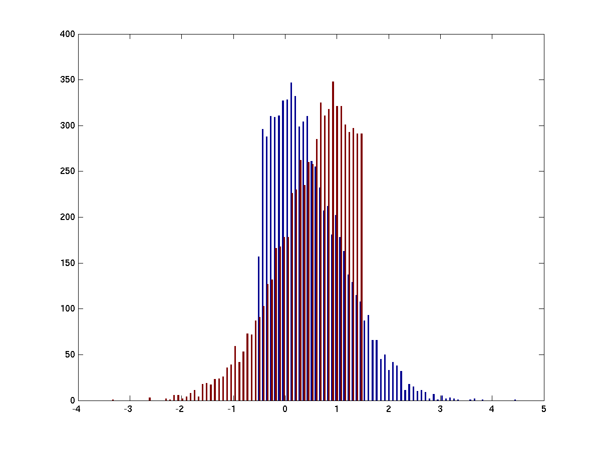
Figure 2

Here we have made the means of the two distributions approximately the same by removing the extreme values of the tails of the two distributions

%%%%%%%%%%%%%%%%%%%%%%%%%%%%%%%%%%%%%%%%%%%%%%%%%%%%%%%%%%%%%%%%%%%%%%%%

s1 = s1_orig;
s2 = s2_orig;

s = [s1(:) s2(:)];
figure; hist(s, 100)

% joint extremes
minval = min([s1 s2]);
maxval = max([s1 s2]);

% create a set of bins
binval = linspace(minval, maxval, 100);

keep1 = false(size(s1));
keep2 = false(size(s2));

for i=1:(length(binval)-1)
  binbeg = binval(i);
  binend = binval(i+1);
  sel1 = find(s1>binbeg & s1<binend);
  sel2 = find(s2>binbeg & s2<binend);
  if length(sel1)>length(sel2)
    % remove some of the trials in s1
    sel1 = sel1(randperm(length(sel1)));
    sel1 = sel1(1:length(sel2));
    keep1(sel1) = true;
    keep2(sel2) = true;
  elseif length(sel1)<length(sel2)
    % remove some of the trials in s2
    sel2 = sel2(randperm(length(sel2)));
    sel2 = sel2(1:length(sel1));
    keep1(sel1) = true;
    keep2(sel2) = true;
  else
    % it is the same number, nothing to do
  end
end

s1 = s1(keep1);
s2 = s2(keep2);

s = [s1(:) s2(:)];
figure; hist(s, 100)

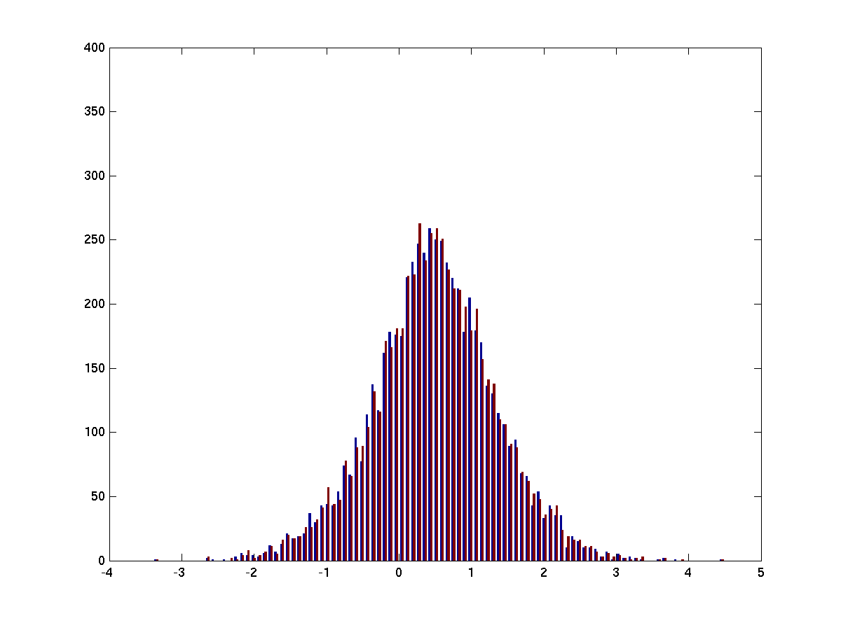
Figure 3

Now we have taken only the part of the two distributions that overlap. Note that this method preserves fewer trials than trimming the extremes.

Note that this easily can be achieved with the FieldTrip ft_stratify function like this

cfg = [];
cfg.method      = 'histogram'
cfg.equalbinavg = 'no';  % 'yes' is more optimal: it also removes the small within-bin bias due to the distributions being shifted
cfg.numbin      = 100;
[strat] = ft_stratify(cfg, s1_orig, s2_orig)

s1    = strat{1};
s2    = strat{2};
% determine which trials to remove from both conditions
keep1 = ~isnan(s1);
keep2 = ~isnan(s2);
s1    = s1(keep1);
s2    = s2(keep2);

% make the same figure as above
s = [s1(:) s2(:)];
figure; hist(s, 100)

Tags: example statistics