Getting started with Biosemi BDF data
Biosemi makes EEG amplifiers for EEG that have active electrodes, i.e the signal is already pre-amplified at the scalp before it is sent to the amplifier box where it is further amplified and digitized. The active electrodes make the recorded signals less sensitive for environmental noise (e.g., electronics noise in the lab) and for movements of the electrode cables. These Biosemi amplifiers are especially popular in applications with high channel density.
The Biosemi system has a few special characteristics
- it uses a non-standard referencing scheme (with the DRL and CMS electrode, rather than GND and REF)
- it stores the data in a 24 bit format
- it uses a sampling rate that is much higher (from 2 kHz upwards) than most EEG systems (commonly around 512 Hz)
- the active electrodes are only useable with electrode caps from Biosemi.
The 24 bit file format has the practical consequence that files are slightly smaller than they would have been when stored with 32-bits, but also that reading and converting the 24 bit numerical representation is very slow because 24 bit is not a standard numerical representation on Intel computers. MATLAB allows to read single bits or 8-bit values from a file, which can be used to construct the 24 bit value, but which is very slow. To speed up the reading, FieldTrip uses a mex file that reads the 24 bit values and converts them to a 32-bit representation on the fly.
The high sampling rate (minimally 2kHz, i.e. 2000 Hz) has the consequence that files are much larger than with most acquisition systems. e.g., when compared to a BrainAmp data file sampled at 512 Hz with the same number of electrodes, the Biosemi data file will be approximately 3x as large on disk and 4x as large after having read it in memory. That means that for processing bdf files you typically will want to have a computer with more than the standard amount of RAM. After reading the data in MATLAB memory, a common procedure is to downsample it to reduce the sampling rate to 500 Hz using ft_resampledata. This will make all subsequent analyses run much faster and will facilitate doing the analysis with less RAM.
Most Biosemi electrode caps have a unique channel naming scheme. Also the exact number and positions is different from those in other EEG systems. Consequently, when plotting the channel-level data with a topographic arrangement of the channels, or when plotting the topographies (see the plotting tutorial and the channel layout tutorial), you will have to use a layout that is specific to your Biosemi electrode cap. FieldTrip includes the following template 2D layout files in the fieldtrip/template/layout directory, but you might want to construct your own layout.
- biosemi16.lay
- biosemi32.lay
- biosemi64.lay
- biosemi128.lay
- biosemi160.lay
- biosemi256.lay
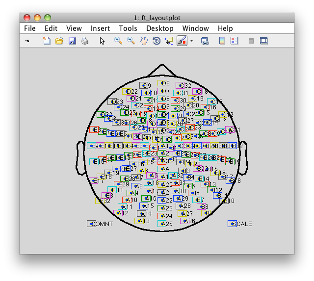
Please note that the use of these layout files requires that the channel labeling in the data is consistent with the channel labeling in the layout file. You might want to check the following
cfg = [];
cfg.layout = 'biosemi160.lay'
ft_layoutplot(cfg)
Referencing Biosemi EEG data
The Biosemi system uses a common-sense (CMS) and a driven-right-leg (DRL) electrode, which injects a small amount of current to minimize the effect of external noise sources. When recording data to disk and when reading it into FieldTrip, it is expressed as potential difference relative to the CMS. With this type of amplifier systems you should always reference after reading the data from disk, i.e. change the reference from CMS to another electrode, and you should not add the CMS electrode as implicit reference channel to the data.
For channel-level analysis you may want to use linked mastoids, or linked T7 and T8. For source analysis you would (as with other systems) best reference to the average of all electrodes (minus CMS).
See also this explanation on the Biosemi website.
Preprocessing and analyzing BDF data
Except for the required referencing, BDF data is processed just like other EEG and MEG data. A simple analysis script would look like this
filename 'yourfile.bdf';

cfg = [];
cfg.dataset = filename;
cfg.trialdef.eventtype  = 'STATUS'
cfg.trialdef.eventvalue = [1 2];
cfg.trialdef.prestim    = 0.2;
cfg.trialdef.poststim   = 0.8;
cfg = ft_definetrial(cfg);

cfg.reref = 'yes';
cfg.refchannel = 'A1';
cfg.demean = 'yes';
cfg.baselinewindow = [-0.2 0];
data = ft_preprocessing(cfg);

cfg = [];
timelock = ft_timelockanalysis(cfg, data);
To find out what the trigger codes are in your BDF file, you can use the following code snippet
event = ft_read_event(filename);

% select only the trigger codes, not the battery and CMS status
sel = find(strcmp({event.type}, 'STATUS'));
event = event(sel);

plot([event.sample], [event.value], '.')
The BDF fileformat
The documentation below is only for reference. To work with this data format you can simply use the standard reading functions ft_read_header, ft_read_data and ft_read_event.
BDF is a 24 bit version of the popular 16 bit EDF format, which was used on previous BioSemi models with 16 bit converters. BDF is almost the same as EDF Although initially the EDF format was mainly used in sleep research, BDF/EDF is now quickly gaining popularity in other EEG applications, ECG body surface potential mapping as well as EMG.
The EDF format was designed and published in 1992 by Bob Kemp, Alpo Värri, Agostinho C. Rosa, Kim D. Nielsen and John Gade as “A simple format for exchange of digitized polygraphic recordings” in Electroencephalography and Clinical Neurophysiology, 82 (1992) 391-393. The original EDF specifications can be found here
Each BDF/EDF file starts with a header followed by the number of Data records indicated in the header.
| Length in bytes | BDF Header | EDF Header | Description |
|---|---|---|---|
| 8 bytes | Byte 1: “255” (non ascii) | Byte 1: “0” (ASCII) | Identification code |
| ::: | Bytes 2-8 : “BIOSEMI” (ASCII) | Bytes 2-8 : “ “(ASCII) | ::: |
| 80 bytes | User text input (ASCII) | Local subject identification | |
| 80 bytes | User text input (ASCII) | Local recording identification | |
| 8 bytes | dd.mm.yy (ASCII) | Startdate of recording | |
| 8 bytes | hh.mm.ss (ASCII) | Starttime of recording | |
| 8 bytes | (ASCII) | Number of bytes in header record | |
| 44 bytes | “24BIT” (ASCII) | “BIOSEMI” (ASCII) | Version of data format |
| 8 bytes | (ASCII) | Number of data records “-1” if unknown | |
| 8 bytes | e.g.: “1” (ASCII) | Duration of a data record, in seconds | |
| 4 bytes | e.g.: “257” or “128”(ASCII) | Number of channels (N) in data record | |
| N x 16 bytes | e.g.: “Fp1”, “Fpz”, “Fp2”, etc (ASCII) | Labels of the channels | |
| N x 80 bytes | e.g.: “active electrode”, “respiration belt” (ASCII) | Transducer type | |
| N x 8 bytes | e.g.: “uV”, “Ohm” (ASCII) | Physical dimension of channels | |
| N x 8 bytes | e.g.: “-262144” (ASCII) | e.g.: “-32768” (ASCII) | Physical minimum in units of physical dimension |
| N x 8 bytes | e.g.: “262143” (ASCII) | e.g.: “32767” (ASCII) | Physical maximum in units of physical dimension |
| N x 8 bytes | e.g.: “-8388608” (ASCII) | e.g.: “-32768” (ASCII) | Digital minimum |
| N x 8 bytes | e.g.: “8388607” (ASCII) | e.g.: “32767” (ASCII) | Digital maximum |
| N x 80 bytes | e.g.: “HP:DC; LP:410” | e.g.: “HP:0,16; LP:500” | Prefiltering |
| N x 8 bytes | For example: “2048” (ASCII) | Number of samples in each data record (Sample-rate if Duration of data record = “1”) | |
| N x 32 bytes | (ASCII) | Reserved |
Bold Text
Number of samples in each data record
(Sample-rate if Duration of data record = “1”)
N x 32 bytes
(ASCII)
Total header length (for BDF and EDF) is: {(N+1)*256} bytes, where N is number of channels (including the status channel).
The “gain” of a specific channel can be calculated by: (Physical max - Physical min) / (Digital max - Digital min). The result is the LSB value in the specified Physical dimension of channels. (31,25nV / 1uV in the BDF/EDF example Header from above).
The last 10 fields are defined for each fields separately. Each channel can be different.
