Frequency analysis of task and resting state EEG

General introduction

In this tutorial we will analyze the power spectra for two different EEG datasets. The first dataset is recorded in a language task, the second dataset is recorded in a resting-state experiment. Before starting with this tutorial, please read through the linked descriptions of the two datasets.

A background on spectral analysis

Oscillatory components contained in the ongoing EEG or MEG signal often change relative to experimental manipulations, such as stimulus events. These oscillatory signals are not necessarily phase-locked to the event and will not be represented as event-related fields (ERFs) in MEG or event-related potentials (ERPs) in EEG (see e.g., Tallon-Baudry and Bertrand (1999) Oscillatory gamma activity in humans and its role in object representation). The goal of the first section is to compute and visualize event-related changes by calculating time-frequency representations (TFRs) of power. This will be done using sliding-window Fourier analysis and by using wavelets.

The sliding-window approach can be done according to two principles: either the window has a fixed length that is independent of frequency, or the time window decreases in length with increased frequency. Prior to calculating the power in the sliding window approach, one or more tapers are multiplied with the data to reduce spectral leakage and control the frequency smoothing.

In the wavelet approach the data is not cut in windows and Fourier transformed, but rather convolved with a wavelet. The Morlet wavelet is constructed by taking a sine (and a cosine) wave at each frequency, and multiplying that with a Gaussian taper. The width of the Gaussian taper is scaled with the frequency, such that there are always a fixed number of cycles in the wavelet, for example 3 or 5.

Figure: Time and frequency smoothing. (a) For a fixed length time window the time and frequency smoothing remains fixed. (b) For time windows that decrease with frequency, the temporal smoothing decreases and the frequency smoothing increases.

If you want to know more about tapers or window functions you can have a look at the time-frequency tutorial. This Wikipedia page explains the effect of the taper or windowing function. Note that Hann window is another name for Hanning window used in this tutorial. There is also a Wikipedia page about multitapers, see here.

Procedure

To compute time-resolved power spectra for the task data and the (non time-resolved) power spectra for the resting state datasets we will perform the following steps:

• Load the data into MATLAB
• Compute the power spectra using ft_freqanalysis
• Visualize the results for all channels and for selected channels. You can make time-frequency plots using ft_singleplotTFR, ft_multiplotTFR and ft_topoplotTFR. For power spectra without time dimension, you can use ft_singleplotER, ft_multiplotER and ft_topoplotER.

Figure: Schematic overview of the steps in time-frequency analysis

Part I: Computing time-frequency representations on task EEG data

TFR with fixed-length windows

Here, we will describe how to calculate time frequency representations using Hanning tapers. When choosing for a fixed window length procedure the frequency resolution is defined according to the length of the time window (delta T). The frequency resolution (delta f in figure 1) = 1/length of time window in sec (delta T in figure 1). Thus a 500 ms time window results in a 2 Hz frequency resolution (1/0.5 sec= 2 Hz) meaning that power can be calculated for 2 Hz, 4 Hz, 6 Hz etc. An integer number of cycles must fit in the time window.

We will skip the preprocessing and start directly with the preprocessed data. You can download data_task.mat from our download server.

load('/madrid2019/tutorial_freq/data_task.mat')

In this tutorial we will pool all stimuli belonging to the visual and auditory categories, forming two datasets: data_visc and data_audc. In the following example a time window with length 500 ms is applied.

cfg              = [];
cfg.output       = 'pow';
cfg.channel      = 'all';
cfg.method       = 'mtmconvol';
cfg.taper        = 'hanning';
cfg.foi          = 2:2:30;                         % analysis 2 to 30 Hz in steps of 2 Hz
cfg.t_ftimwin    = ones(length(cfg.foi),1).*0.5;   % length of time window = 0.5 sec
cfg.toi          = -1:0.05:1;                      % the time window "slides" from -0.5 to 1.5 in 0.05 sec steps
TFRhann_visc = ft_freqanalysis(cfg, data_visc);    % visual stimuli
TFRhann_audc = ft_freqanalysis(cfg, data_audc);    % auditory stimuli

Irrespective of the method used for calculating the TFR, the output format is identical. It is a structure with the following element

TFRhann_visc =

      label: {64x1 cell}                 % Channel names
     dimord: 'chan_freq_time'            % Dimensions contained in powspctrm, channels X frequencies X time
       freq: [2 4 6 8 10 12 14 16 18 20 22 24 26 28 30]  % Array of frequencies of interest (the elements of freq may be different from your cfg.foi input depending on your trial length)
       time: [1x41 double]               % Array of time points considered
  powspctrm: [64x15x41 double]           % 3-D matrix containing the power values
        cfg: [1x1 struct]                % Settings used in computing this frequency decomposition

The field TFRhann_visc.powspctrm contains the power for each channel, for each frequency and for each time point.

Visualization

This part of the tutorial shows how to visualize the results of any type of time-frequency analysis.

To make the changes in the event-related power better visible, we will normalization the power with respect to a baseline interval. There are multiple ways that you can normalize (see ft_freqbaseline), the most common two are (a) subtracting, for each frequency, the average power in the baseline interval from the power at all time points. This gives the absolute change in power with respect to the baseline interval. Another method is (b) dividing, for each frequency, the power at all time points by the average power in the baseline interval. This gives the relative increase (or relative decrease) of the power at all frequencies and time points with respect to the power in the baseline interval. Note that the relative baseline is expressed as a ratio; i.e. no change is represented by 1.

There are three ways of graphically representing the data: 1) time-frequency plots of all channels, in a quasi-topographical layout, 2) time-frequency plot of an individual channel (or the average of several channels), 3) topographical 2-D map of the power changes in a specified time-frequency interval.

To plot the TFRs from all the sensors use the function ft_multiplotTFR. Settings can be adjusted in the cfg structure. For example:

    cfg = [];
    cfg.baseline     = [-0.5 -0.3];
    cfg.baselinetype = 'absolute';
    cfg.showlabels   = 'yes';
    cfg.layout       = 'easycapM10.mat';
    figure; ft_multiplotTFR(cfg, TFRhann_visc);

Figure: Time-frequency representations calculated using ft_freqanalysis. Plotting was done with ft_multiplotTFR)

By using the options cfg.baseline and cfg.baselinetype in the call to the plotting functions, the baseline correction is applied on the fly. Baseline correction can also be applied by calling ft_freqbaseline.

You can combine the various visualization options/functions interactively to explore your data by clicking and dragging with your mouse in the window. See also the plotting tutorial for more details.

An interesting effect seems to be present in the TFR of channel 1. To make a plot of a single channel use the function ft_singleplotTFR

    cfg = [];
    cfg.baseline     = [-0.5 -0.3];
    cfg.baselinetype = 'absolute';
    cfg.maskstyle    = 'saturation';
    cfg.zlim         = [0 20];
    cfg.channel      = '1';
    cfg.layout       = 'easycapM10.mat';

    figure;
    subplot(211); ft_singleplotTFR(cfg, TFRhann_visc); title('visual stim');
    subplot(212); ft_singleplotTFR(cfg, TFRhann_audc); title('auditory stim');

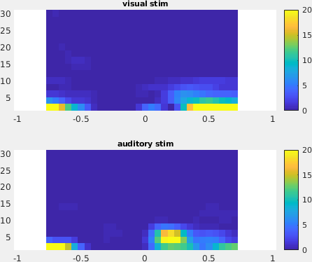
Figure: The time-frequency representation with respect to single sensor obtained using ft_singleplotTFR.

If you see plotting artifacts in your figure, see this question.

From the figure, you can see that there is an increase in power around 3-8 Hz in the time interval 0.1 to 0.3 s after stimulus onset. To show the topography of this power increase use the function ft_topoplotTFR

    cfg = [];
    cfg.baseline     = [-0.5 -0.3];
    cfg.baselinetype = 'absolute';
    cfg.xlim         = [0.1 0.3];
    cfg.zlim         = [0 10];
    cfg.ylim         = [3 8];
    cfg.marker       = 'on';
    cfg.layout       = 'easycapM10.mat';
    figure;
    subplot(211);ft_topoplotTFR(cfg, TFRhann_visc); title('visual stim');
    subplot(212);ft_topoplotTFR(cfg, TFRhann_audc); title('auditory stim');

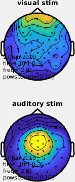
Figure: A topographic representation of the time-frequency representations (3 - 8 Hz, 0.1 - 0.3 s post stimulus) obtained using ft_topoplotTFR

Exercise 1

Exercise 2

TFR with Morlet wavelets

An alternative to calculating TFRs with sliding windows is to use Morlet wavelets. This approach is very similar to calculating TFRs with time windows that depend on the frequency and using a Gaussian taper. The commands below illustrate how to do this. One crucial parameter to set is cfg.width. It determines the width of the wavelets in number of cycles. Making the value smaller will increase the temporal resolution at the expense of frequency resolution and vice versa. The spectral bandwidth at a given frequency F is equal to F/width2 (so, at 30 Hz and a width of 7, the spectral bandwidth is 30/72 = 8.6 Hz) while the wavelet duration is equal to width/F/pi (in this case, 7/30/pi = 0.074s = 74ms).

Calculate TFRs using Morlet wavelet

cfg = [];
cfg.channel    = 'all';
cfg.method     = 'wavelet';
cfg.width      = 7;
cfg.output     = 'pow';
cfg.foi        = 1:2:30;
cfg.toi        = -1:0.05:1;
TFRwave_visc = ft_freqanalysis(cfg, data_visc);    % visual stimuli
TFRwave_audc = ft_freqanalysis(cfg, data_audc);    % auditory stimuli

Plot the result

cfg = [];
cfg.baseline     = [-0.5 -0.3];
cfg.baselinetype = 'absolute';
cfg.marker       = 'on';
cfg.layout       = 'easycapM10.mat';
cfg.channel      = '1';
cfg.interactive  = 'no';
figure;
subplot(211);ft_singleplotTFR(cfg, TFRwave_visc); title('visual stim');
subplot(212);ft_singleplotTFR(cfg, TFRwave_audc); title('auditory stim');

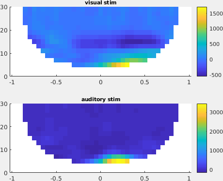
Figure: Time-frequency representations of power calculated using Morlet wavelets.

Exercise 3

If you would like to learn more about plotting of time-frequency representations, please see the visualization section or the plotting tutorial.

Part II: Spectral analysis on EEG resting state data

In the remainder of this tutorial we will be analyzing the EEG data from an single subject from the Chennu et al. dataset, specifically the baseline session from participant 22. As it is a resting state recording, we assume that the power spectrum is stationary (i.e. constant) over time, hence we will only look at the spectrum in the frequency domain averaged for the whole duration of the recording, not how it changes over times.

We will skip the preprocessing and start directly with the preprocessed data. You can download data_rest.mat from our download server.

clear all, close all, clc
load data_rest.mat

Effect of the window length

We read the data of participant 22 (baseline sedation session) and we will use ft_redefinetrial to cut shorter trials out of the continuous data. Specifically, we will cut the data into non-overlapping segments of various lengths (1 sec, 2 secs and 4 secs) and we will compute the power spectrum of all data segments and average them.

cfg1 = [];
cfg1.length  = 1;
cfg1.overlap = 0;
base_rpt1    = ft_redefinetrial(cfg1, base);

cfg1.length  = 2;
base_rpt2    = ft_redefinetrial(cfg1, base);

cfg1.length  = 4;
base_rpt4    = ft_redefinetrial(cfg1, base);

Now we use ft_freqanalysis to compute the power spectra using a boxcar window

cfg2 = [];
cfg2.output  = 'pow';
cfg2.channel = 'all';
cfg2.method  = 'mtmfft';
cfg2.taper   = 'boxcar';
cfg2.foi     = 0.5:1:45; % 1/cfg1.length  = 1;
base_freq1   = ft_freqanalysis(cfg2, base_rpt1);

cfg2.foi     = 0.5:0.5:45; % 1/cfg1.length  = 2;
base_freq2   = ft_freqanalysis(cfg2, base_rpt2);

cfg2.foi     = 0.5:0.25:45; % 1/cfg1.length  = 4;
base_freq4   = ft_freqanalysis(cfg2, base_rpt4);

Let us plot the power spectra of channel 61 using the standard MATLAB plot function.

figure;
hold on;
plot(base_freq1.freq, base_freq1.powspctrm(61,:))
plot(base_freq2.freq, base_freq2.powspctrm(61,:))
plot(base_freq4.freq, base_freq4.powspctrm(61,:))
legend('1 sec window','2 sec window','4 sec window')
xlabel('Frequency (Hz)');
ylabel('absolute power (uV^2)');

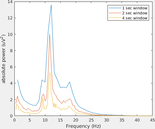
Note the differences in power and in frequency resolution for each window length.

Can you explain why the amplitude of the power spectra decrease increasing the window length? Hint: think of the stationarity assumption in FFT

Effect of different tapers

Finally, we will look at the effect of different tapers on the power estimates. To enhance the effects of the tapers, we will use the data chopped in windows of 4 seconds. So let us run again ft_freqanalysis but this time using different tapers: boxcar, Hanning and discrete prolate spheroidal sequences (DPSS, i.e. multitapers).

But before doing anything, let us recapitulate what multitapers are good for? Multitapers are typically used to achieve better control over the frequency smoothing. More tapers for a given time window will result in greater smoothing. High frequency smoothing is particularly advantageous when dealing with electrophysiological brain signals above 30 Hz. Oscillatory gamma activity (30-100 Hz) is quite broad band and thus analysis of such signals benefit from multitapering. For signals lower than 30 Hz it is recommend to use only a single taper, e.g., a Hanning taper as shown above. Beware that in the example below multitapers are used to analyze low frequencies, because there are no gamma band effects in this particular dataset.

Spectral analysis with on multitapers is done with the function ft_freqanalysis. The function uses the time in which the data has been segmented during preprocessing. Prior to the Fourier transformations, the data are “tapered”. A single taper can be applied (e.g. Hanning) or several orthogonal tapers might be used for each time window (e.g. DPSS). The power is calculated for each tapered data segment and then averaged over tapers. In the example below we already have the data segmented in windows of different sizes (1, 2, 4 seconds) and we can compute the power spectra using the following parameters:

• cfg.foi determines the frequencies of interest, here from 1 Hz to 30 Hz in steps of 2 Hz. The step size could be decreased at the expense of computation time and redundancy.

• cfg.tapsmofrq determines the width of frequency smoothing in Hz (= fw). We have chosen cfg.tapsmofrq = 4, which assumes a bandwidth of 8Hz smoothing (±4). For less smoothing you can specify smaller values, however, the following relation determined by the Shannon number must hold (see Percival and Walden (1993)):

K = 2*tw*fw-1, where K is required to be larger than 0.

K is the number of tapers applied; the more, the greater the smoothing.

cfg2 = [];
cfg2.output    = 'pow';
cfg2.channel   = 'all';
cfg2.method    = 'mtmfft';
cfg2.taper     = 'boxcar';
cfg2.foi       = 0.5:0.25:45;
base_freq_b    = ft_freqanalysis(cfg2, base_rpt4);

cfg2.taper     = 'hanning';
base_freq_h    = ft_freqanalysis(cfg2, base_rpt4);

cfg2.taper     = 'dpss'; % here the multitapers
cfg2.tapsmofrq = 4;
base_freq_d    = ft_freqanalysis(cfg2, base_rpt4);

figure; hold on
plot(base_freq_b.freq, base_freq_b.powspctrm(61,:))
plot(base_freq_h.freq, base_freq_h.powspctrm(61,:))
plot(base_freq_d.freq, base_freq_d.powspctrm(61,:))
legend('4 sec boxcar', '4 secs hanning', '4 sec dpss');
xlabel('Frequency (Hz)');
ylabel('absolute power (uV^2)');

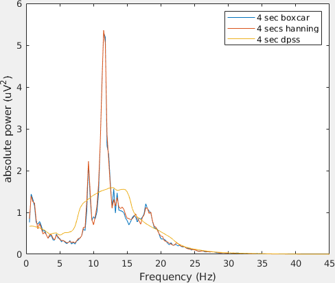
Note the differences in amplitude and frequency resolution for each taper, specially the DPSS. Can you explain why the amplitude of the power spectra decrease that much given that in this case the non-stationarity of the data is the same across tapers?

Changes in power due to propofol sedation

Finally, we will apply what we just learned to investigate the experimental effect of propofol on the resting-state EEG power spectrum.

cfg1 = [];
cfg1.length  = 4;
cfg1.overlap = 0;
mild_rpt4 = ft_redefinetrial(cfg1, mild);
mode_rpt4 = ft_redefinetrial(cfg1, mode);
reco_rpt4 = ft_redefinetrial(cfg1, reco);

cfg2 = [];
cfg2.output  = 'pow';
cfg2.channel = 'all';
cfg2.method  = 'mtmfft';
cfg2.taper   = 'boxcar';
cfg2.foi     = 0.5:0.25:45;
mild_freq_b  = ft_freqanalysis(cfg2, mild_rpt4);
mode_freq_b  = ft_freqanalysis(cfg2, mode_rpt4);
reco_freq_b  = ft_freqanalysis(cfg2, reco_rpt4);

cfg2.taper   = 'hanning';
mild_freq_h  = ft_freqanalysis(cfg2, mild_rpt4);
mode_freq_h  = ft_freqanalysis(cfg2, mode_rpt4);
reco_freq_h  = ft_freqanalysis(cfg2, reco_rpt4);

cfg2.taper   = 'dpss';
cfg2.tapsmofrq = 4;
mild_freq_d  = ft_freqanalysis(cfg2, mild_rpt4);
mode_freq_d  = ft_freqanalysis(cfg2, mode_rpt4);
reco_freq_d  = ft_freqanalysis(cfg2, reco_rpt4);

figure; ft_multiplotER([], base_freq_b, mild_freq_b, mode_freq_b, reco_freq_b)
figure; ft_multiplotER([], base_freq_h, mild_freq_h, mode_freq_h, reco_freq_h)
figure; ft_multiplotER([], base_freq_d, mild_freq_d, mode_freq_d, reco_freq_d)

Which set of parameters are more sensitive to detect the spectrum shift (increase of low beta power)?