FieldTrip connectivity demo

%% start with data that was preprocessed in FieldTrip
subj = 15;
prefix = sprintf('Sub%02d', subj);
load([prefix '_raw']);  % this is called "data" rather than "raw"

% load the results from beamformer_part1
load vol
load sens
load mri_realigned


%% deal with maxfilter

% the data has been maxfiltered and subsequently contatenated
% this results in an ill-conditioned estimate of covariance or CSD

cfg             = [];
cfg.method      = 'pca';
cfg.updatesens  = 'no';
cfg.channel     = 'MEGMAG';
comp = ft_componentanalysis(cfg, data);

cfg             = [];
cfg.updatesens  = 'no';
cfg.component   = comp.label(51:end);
data_fix = ft_rejectcomponent(cfg, comp);


%%

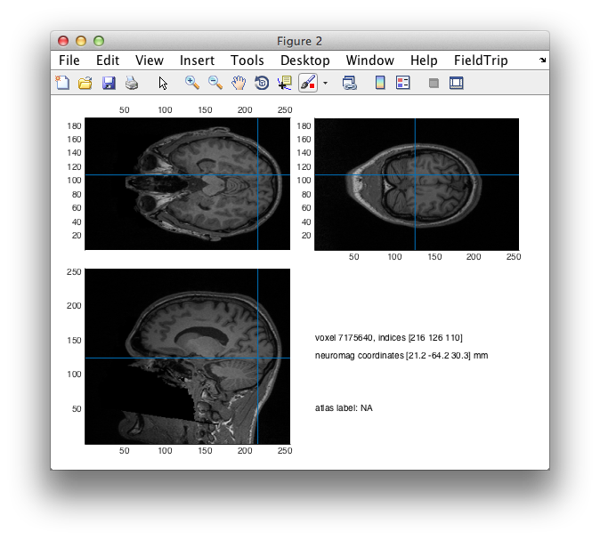
pos1 = [21 -64 30];
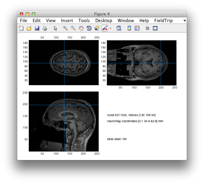
pos2 = [0 35 83];

cfg = [];
cfg.location = pos1;
figure; ft_sourceplot(cfg, mri_realigned);
cfg.location = pos2;
figure; ft_sourceplot(cfg, mri_realigned);

%%
% timelock2 was computed in https://www.fieldtriptoolbox.org/workshop/meg-uk-2015/fieldtrip-beamformer-demo#part_3_-_reconstruct_single-trial_cortical_responses

cfg             = [];
cfg.headmodel   = vol;
cfg.grad        = sens;
cfg.senstype    = 'meg';
cfg.method      = 'lcmv';
cfg.lcmv.keepfilter = 'yes';
cfg.lcmv.projectmom = 'yes';
cfg.unit   = 'mm';
cfg.sourcemodel.pos    = pos1;
source1 = ft_sourceanalysis(cfg, timelock2);

cfg.sourcemodel.pos = pos2;
source2 = ft_sourceanalysis(cfg, timelock2);


%% construct single-trial virtual channel representation

virtualchannel_raw = [];
virtualchannel_raw.label = {'pos1'; 'pos2'};
virtualchannel_raw.trialinfo = data_fix.trialinfo;
for i=1:882
% note that this is the non-filtered raw data
virtualchannel_raw.time{i}       = data_fix.time{i};
virtualchannel_raw.trial{i}(1,:) = source1.avg.filter{1} * data_fix.trial{i}(:,:);
virtualchannel_raw.trial{i}(2,:) = source2.avg.filter{1} * data_fix.trial{i}(:,:);
end

%%

cfg                 = [];
cfg.keeptrials      = 'yes';
cfg.preproc.demean  = 'yes';
cfg.preproc.baselinewindow = [-inf 0];
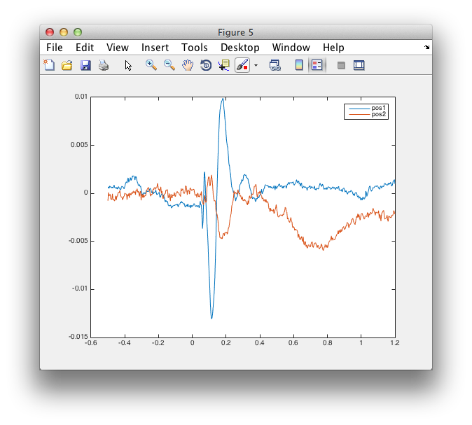
virtualchannel_avg = ft_timelockanalysis(cfg, virtualchannel_raw);

figure
plot(virtualchannel_avg.time, virtualchannel_avg.avg)
legend(virtualchannel_avg.label);

%%

cfg         = [];
cfg.method  = 'wavelet';
cfg.output  = 'powandcsd';
cfg.foi     = 4:2:70;
cfg.toi     = -0.200:0.020:1.000;
virtualchannel_wavelet = ft_freqanalysis(cfg, virtualchannel_raw);

cfg                 = [];
cfg.baselinetype    = 'relative';
cfg.baseline        = [-inf 0];
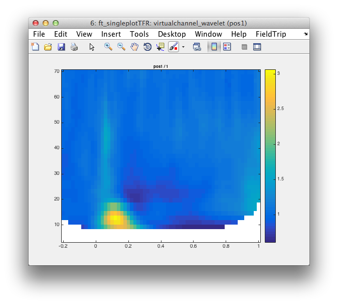
cfg.channel         = {'pos1'};
figure; ft_singleplotTFR(cfg, virtualchannel_wavelet);

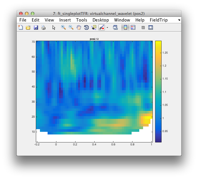
cfg.channel         = {'pos2'};
figure; ft_singleplotTFR(cfg, virtualchannel_wavelet);

%%

cfg = [];
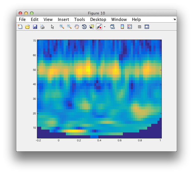
cfg.method = 'coh';
coherence = ft_connectivityanalysis(cfg, virtualchannel_wavelet);


figure
imagesc(coherence.time, coherence.freq, squeeze(coherence.cohspctrm(1,:,:)));
axis xy

%% start from data that was processed by FieldTrip
subj = 15;
prefix = sprintf('Sub%02d', subj);
load([prefix '_raw']);  % this is called "data" rather than "raw"

% load the results from beamformer_part1
load vol
load sens
load mri_realigned


%% deal with maxfilter

% the data has been maxfiltered and subsequently contatenated
% this results in an ill-conditioned estimate of covariance or CSD

cfg = [];
cfg.method = 'pca';
cfg.updatesens = 'no';
cfg.channel = 'MEGMAG';
comp = ft_componentanalysis(cfg, data);

cfg = [];
cfg.updatesens = 'no';
cfg.component = comp.label(51:end);
data_fix = ft_rejectcomponent(cfg, comp);

%%

cfg = [];
cfg.channel = 'MEGMAG';
cfg.method = 'wavelet';
cfg.output = 'fourier';
cfg.keeptrials = 'yes';
cfg.foi = 16;
cfg.toi = 0.150;
freq = ft_freqanalysis(cfg, data_fix);


%%

cfg = [];
cfg.resolution = 7;
% cfg.inwardshift = -7; % allow dipoles 10mm outside the brain, this improves interpolation at the edges
cfg.unit = 'mm';
cfg.headmodel = vol;  % from FT
cfg.grad      = sens; % from FT
cfg.senstype  = 'meg';
cfg.normalize = 'yes';
grid = ft_prepare_leadfield(cfg, freq);

% save grid grid


%%

cfg           = [];
cfg.headmodel = vol;  % from FT
cfg.grad      = sens; % from FT
cfg.senstype  = 'meg';
cfg.grid      = grid;
cfg.method    = 'pcc';
cfg.pcc.fixedori = 'yes';
cfg.latency   = [0.140 0.160];
cfg.frequency = [14 18];

source = ft_sourceanalysis(cfg, freq);

figure
plot(source.avg.mom{source.inside(1)}, '.')
xlabel('real');
ylabel('imag');

%%

pos = [21 -64 30];

% compute the nearest grid location
dif = grid.pos;
dif(:,1) = dif(:,1)-pos(1);
dif(:,2) = dif(:,2)-pos(2);
dif(:,3) = dif(:,3)-pos(3);
dif = sqrt(sum(dif.^2,2));
[distance, refindx] = min(dif);

cfg = [];
cfg.method    = 'coh';
% cfg.complex   = 'abs';
cfg.complex   = 'absimag';
cfg.refindx   = refindx;
conn = ft_connectivityanalysis(cfg, source);

% the output contains both the actual source position, as well as the position of the reference
% this is ugly and will probably change in future FieldTrip versions
orgpos = conn.pos(:,1:3);
refpos = conn.pos(:,4:6);
conn.pos = orgpos;

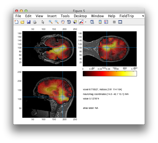
%% visualise the seed-based connectivity results

cfg               = [];
cfg.funparameter  = 'cohspctrm';
figure; ft_sourceplot(cfg, conn);

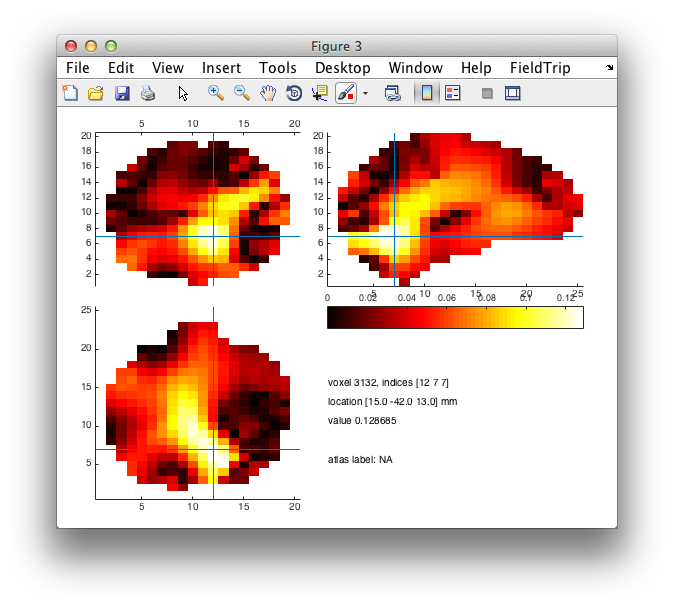
cfg             = [];
cfg.parameter   = 'cohspctrm';
sourceI = ft_sourceinterpolate(cfg, conn, mri_realigned);

cfg               = [];
cfg.funparameter  = 'cohspctrm';
figure; ft_sourceplot(cfg, sourceI);

%% look at connectivity difference

cfg         = [];
cfg.trials  = find(freq.trialinfo==1 | freq.trialinfo==2); % 1=Famous, 2=Unfamiliar
source1 = ft_selectdata(cfg, source);

cfg.trials  = find(freq.trialinfo==3); % 3=Scrambled
source2 = ft_selectdata(cfg, source);

% consider using ft_stratify to equalise number of trials going in to source 1 and 2, as SNR differences between conditions affects connectivity measures between conditions

cfg         = [];
cfg.method  = 'coh';
cfg.complex = 'absimag';
cfg.refindx = refindx;
conn1 = ft_connectivityanalysis(cfg, source1);
conn2 = ft_connectivityanalysis(cfg, source2);

conn1.pos = conn1.pos(:,1:3);
conn2.pos = conn2.pos(:,1:3);

cfg           = [];
cfg.parameter = 'cohspctrm';
cfg.operation = 'x1-x2'; % or 'subtract'
conn_dif = ft_math(cfg, conn1, conn2);

cfg           = [];
cfg.parameter = 'cohspctrm';
source1int    = ft_sourceinterpolate(cfg, conn1, mri_realigned);
source2int    = ft_sourceinterpolate(cfg, conn2, mri_realigned);
source_difint = ft_sourceinterpolate(cfg, conn_dif, mri_realigned);

cfg               = [];
cfg.funparameter  = 'cohspctrm';
cfg.funcolorlim   = [-0.1 0.1];
cfg.maskparameter = 'cohspctrm';
cfg.opacitylim    = [-0.15 0.15];
figure; ft_sourceplot(cfg, source_difint);

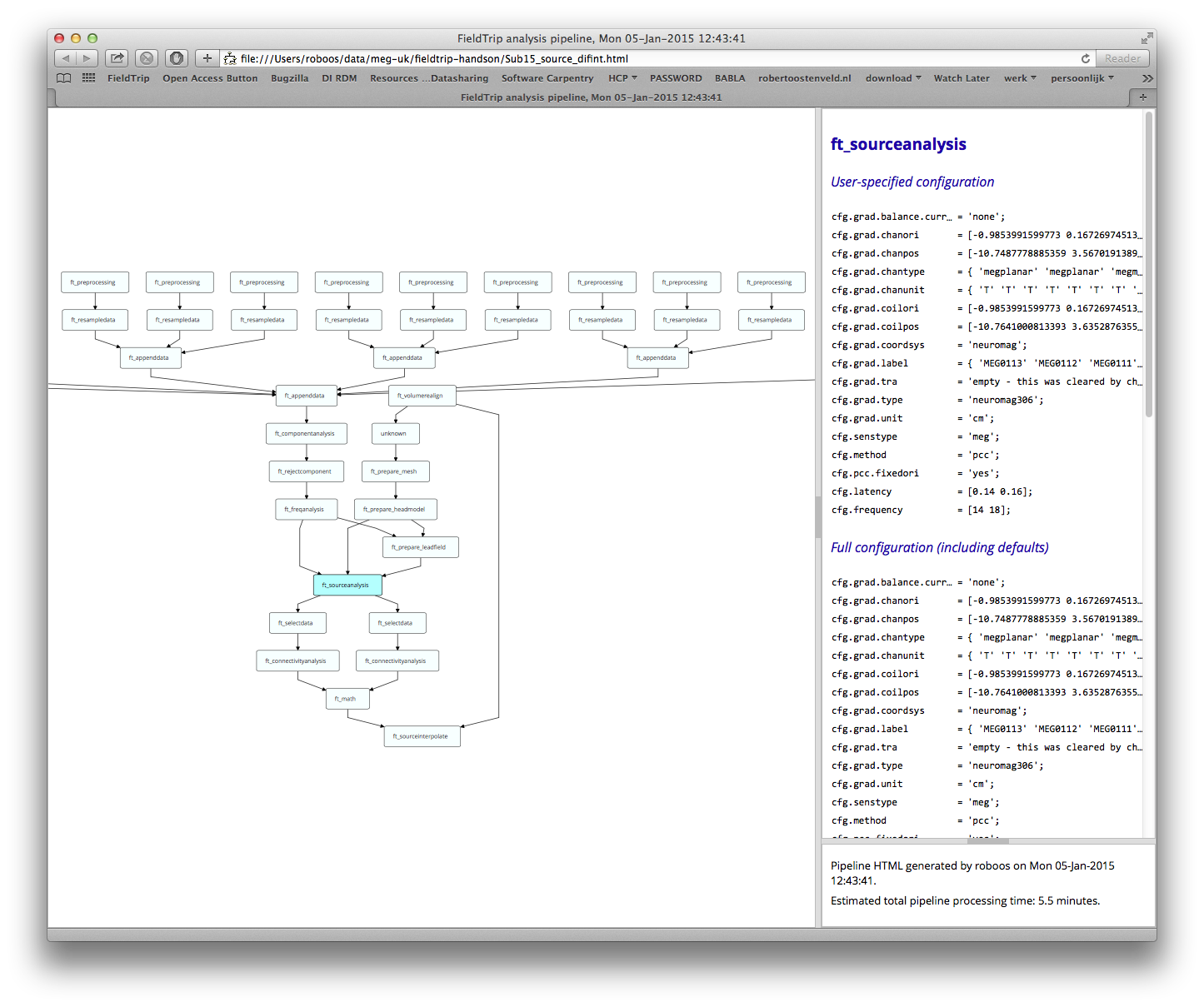
%% look at the analysis history

% for saving to disk
prefix = sprintf('Sub%02d', subj);

cfg           = [];
cfg.filename  = [prefix '_source_difint.html'];
ft_analysispipeline(cfg, source_difint);