From raw data to ERP

Introduction

In this tutorial, we will learn how to read in ‘raw’ data from a file, and to apply some basic processing and averaging in order to inspect event-related fields.

Preliminaries, definition of subject specific filenames, and definition of epochs-of-interest

In FieldTrip the preprocessing of data refers to the reading of the data, segmenting the data around interesting events such as triggers, temporal filtering and optionally rereferencing. The ft_preprocessing function takes care of all these steps, i.e., it reads the data and applies the preprocessing options.

There are largely two alternative approaches for preprocessing, which especially differ in the amount of memory required. The first approach is to read all data from the file into memory, apply filters, and subsequently cut the data into interesting segments. The second approach is to first identify the interesting segments, read those segments from the data file and apply the filters to those segments only. The remainder of this tutorial explains the second approach, as that is the most appropriate for large data sets such as the MEG data used in this tutorial. The approach for reading and filtering continuous data and segmenting afterwards is explained in another tutorial.

Preprocessing involves several steps including defining epochs-of-interest from the dataset, filtering and artifact rejections. This tutorial covers how to identify epochs based on the recorded events during the experiment. Typically, this requires the use of ft_definetrial. For more details, see the preprocessing tutorial.

The output of ft_definetrial is a configuration structure containing the field cfg.trl. This is a matrix representing the relevant parts of the raw datafile which are to be selected for further processing. Each row in the trl matrix represents a single epoch-of-interest, and the trl matrix has at least 3 columns. The first column defines (in samples) the begin of each epoch with respect to how the data are stored in the raw datafile. The second column defines (in samples) the end of each epoch, and the third column specifies the offset (in samples) of the first sample within each epoch with respect to timepoint 0 within that epoch.

In this tutorial, we will bypass ft_definetrial altogether, and create a trl matrix ‘by hand’, using information obtained from the ‘events.tsv’ files, which contain the necessary event information, specifically which type of stimulus was presented when. In order to extract the events from a given dataset, FieldTrip has the function ft_read_event. Each event in the output structure is of a particular type (and may have a specific value), and has an associated sample, which reflects the time point expressed in samples relative to the onset of the data recording. According to BIDS, event timing is expressed in units of time in the events.tsv file, and in order to express the event timing in samples, information about the sampling frequency (which is present in the header information of the dataset) needs to be passed into the function as well.

First, to get started, we need to know which files to use. One way to do this, is to work with a subject specific text file that contains this information. Alternatively, in MATLAB, we can represent this information in a subject-specific data structure, where the fields contain the filenames of the files (including the directory) that are relevant. Here, we use the latter strategy. We use the datainfo_subject function, which is provided in the code folder associated with this workshop. If we do the following:

subj = datainfo_subject(15);

We obtain a structure that looks like this:

 subj =

 struct with fields:

             id: 15
           name: 'sub-15'
        mrifile: '/project_qnap/3010000.02/practicalMEEG/ds00011?'
        fidfile: '/project_qnap/3010000.02/practicalMEEG/ds00011?'
     outputpath: '/project_qnap/3010000.02/practicalMEEG/process?'
        megfile: {6x1 cell}
     eventsfile: {6x1 cell}

We can now run the following chunk of code:

trl = cell(6,1);
for run_nr = 1:6
  hdr   = ft_read_header(subj.megfile{run_nr});
  event = ft_read_event(subj.eventsfile{run_nr}, 'header', hdr, 'eventformat', 'bids_tsv');

  trialtype = {event.type}';
  sel       = ismember(trialtype, {'Famous' 'Unfamiliar' 'Scrambled'});
  event     = event(sel);

  prestim  = round(0.5.*hdr.Fs);
  poststim = round(1.2.*hdr.Fs-1);

  trialtype = {event.type}';
  trialcode = nan(numel(event),1);
  trialcode(strcmp(trialtype, 'Famous'))     = 1;
  trialcode(strcmp(trialtype, 'Unfamiliar')) = 2;
  trialcode(strcmp(trialtype, 'Scrambled'))  = 3;

  begsample = max(round([event.sample]) - prestim,  1);
  endsample = min(round([event.sample]) + poststim, hdr.nSamples);
  offset    = -prestim.*ones(numel(begsample),1);

  subj.trl{run_nr} = [begsample(:) endsample(:) offset(:) trialcode(:) ones(numel(begsample),1).*run_nr];
  clear trl;
end

Reading in raw data from disk

In the section above, we have created a set of trl matrices, which contain, for each of the runs in the experiment, a specification of the begin, and endpoint of the relevant epochs. We can now proceed with reading in the data, applying a bandpass filter, and excluding filter edge effects in the data-of-interest, by using the cfg.padding argument. The below chunk of code takes some time (and RAM) to compute, so if your computer is not up to this, you can also skip this step, and load in the sub-15_data.mat from the derivatives/raw2erp/sub-15 folder:

  rundata = cell(1,6);
  for run_nr = 1:6

    cfg         = [];
    cfg.dataset = subj.megfile{run_nr};
    cfg.trl     = subj.trl{run_nr};

    % MEG specific settings
    cfg.channel = 'MEG';
    cfg.demean  = 'yes';
    cfg.coilaccuracy = 0;
    cfg.bpfilter = 'yes';
    cfg.bpfilttype = 'firws';
    cfg.bpfreq  = [1 40];
    cfg.padding = 3;
    data_meg    = ft_preprocessing(cfg);

    % EEG specific settings
    cfg.channel    = {'EEG' '-EEG061' '-EEG062' '-EEG063' '-EEG064'};
    cfg.demean     = 'yes';
    cfg.reref      = 'yes';
    cfg.refchannel = 'all'; % average reference
    data_eeg       = ft_preprocessing(cfg);

    % settings for all other channels
    cfg.channel = {'all', '-MEG', '-EEG'};
    cfg.demean  = 'no';
    cfg.reref   = 'no';
    cfg.bpfilter = 'no';
    data_other  = ft_preprocessing(cfg);

    cfg            = [];
    cfg.resamplefs = 300;
    data_meg       = ft_resampledata(cfg, data_meg);
    data_eeg       = ft_resampledata(cfg, data_eeg);
    data_other     = ft_resampledata(cfg, data_other);

    %% append the different channel sets into a single structure
    rundata{run_nr} = ft_appenddata([], data_meg, data_eeg, data_other);
    clear data_meg data_eeg data_other
  end % for each run

  data = ft_appenddata([], rundata{:});
  clear rundata;

  filename = fullfile(subj.outputpath, 'raw2erp', sprintf('%s_data',  subj.name));
  % save(filename, 'data');
  % load(filename, 'data');

The above chunk of code uses ft_preprocessing three times per run, with channel type specific processing options. Of note is the rereferencing of the EEG data, and the exclusion of a subset of the EEG channels. The excluded channels correspond to non-brain recording EEG signals (EOG/ECG etc.), and are excluded from further analysis. Subsequently, the EEG data are average-referenced. After the data has been read from disk, ft_resampledata is used to downsample the data to a sampling frequency of 300 Hz. Then, the data structures are combined into a single run-specific data structure, using ft_appenddata.

Compute condition-specific averages (ERFs/ERPs)

Once the data has been epoched and filtered, we can proceed with computing event-related averages. In FieldTrip, this can be achieved with ft_timelockanalysis. In order to selectively average across epochs from different conditions, we make use of the data.trialinfo field, which contains a numeric indicator of the condition to which that particular epoch belongs. Thus, we can do:

cfg        = [];
cfg.trials = find(data.trialinfo(:,1)==1);
cfg.preproc.demean = 'yes';
cfg.preproc.baselinewindow = [-0.1 0];
avg_famous = ft_timelockanalysis(cfg, data);
cfg.trials = find(data.trialinfo(:,1)==2);
avg_unfamiliar = ft_timelockanalysis(cfg, data);

cfg.trials = find(data.trialinfo(:,1)==3);
avg_scrambled = ft_timelockanalysis(cfg, data);

cfg.trials = find(data.trialinfo(:,1)==1 | data.trialinfo(:,1)==2);
avg_faces  = ft_timelockanalysis(cfg, data);

filename = fullfile(subj.outputpath, 'raw2erp', sprintf('%s_timelock', subj.name));
% save(filename, 'avg_famous', 'avg_unfamiliar', 'avg_scrambled', 'avg_faces');
% load(filename, 'avg_famous', 'avg_unfamiliar', 'avg_scrambled', 'avg_faces');

Visualisation of the ERFs

At this stage, we have a set of spatiotemporal matrices, reflecting the electrophysiological response to different types of stimuli. In order to visualise the time courses, and interpret the spatial distribution of the responses, we can use a combination of the following FieldTrip functions: ft_multiplotER, ft_topoplotER, ft_singleplotER. With the exception of ft_singleplotER these functions require a specification of (a 2D projection) of the positions of the sensors/electrodes. In FieldTrip, this is specified by the cfg.layout option; you can read more about this in the layout tutorial. More information about the visualisation of sensor (and source) level data can be found in the plotting tutorial.

Each type of channel can be visualised with its corresponding layout. For the visualisation of the gradiometers, we first compute the magnitude of the gradient by combining the ‘horizontal’ and ‘vertical’ gradients at each sensor location, using ft_combineplanar.

% visualise the magnetometer data
cfg        = [];
cfg.layout = 'neuromag306mag_helmet.mat';
figure; ft_multiplotER(cfg, avg_famous, avg_unfamiliar, avg_scrambled);

% combine planar gradients and visualise the gradiometer data
cfg              = [];
avg_faces_c      = ft_combineplanar(cfg, avg_faces);
avg_famous_c     = ft_combineplanar(cfg, avg_famous);
avg_unfamiliar_c = ft_combineplanar(cfg, avg_unfamiliar);
avg_scrambled_c  = ft_combineplanar(cfg, avg_scrambled);

cfg        = [];
cfg.layout = 'neuromag306cmb_helmet.mat';
figure; ft_multiplotER(cfg, avg_famous_c, avg_unfamiliar_c, avg_scrambled_c);

% create an EEG channel layout on-the-fly and visualise the eeg data
cfg      = [];
cfg.elec = avg_faces.elec;
layout_eeg = ft_prepare_layout(cfg);

cfg        = [];
cfg.layout = layout_eeg;
figure; ft_multiplotER(cfg, avg_famous, avg_unfamiliar, avg_scrambled);

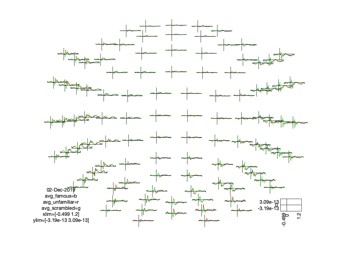
Figure: Distribution of magnetometer ERFs on a 2D projected sensory layout.

The figure that is generated by ft_multiplotER shows in a spatial distribution the ERFs on the different channels (in this case: magnetometers). The figure is interactive, and you can select subsets of channels by drawing a rectangle in the figure panel, followed by a left mouse click. This results in a figure that shows the condition specific ERFs as an average across the selected sensors. This representation is the same as when using ft_singleplotER. Selecting a time range in this figure results in a set of condition specific figures that show the topographical distribution of the ERF amplitude, as an average across the selected latency window.

Figure: Average across selected magnetometers for each of the conditions.

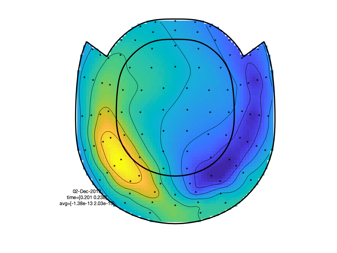
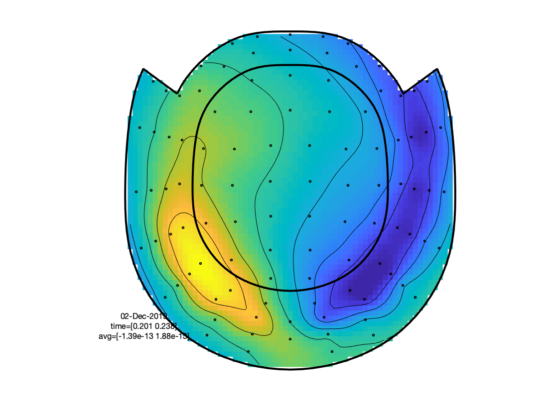
Figure: Topographies of average across selected latency window for each of the conditions.

Alternatively, the data of different channel types can be visualised within a single figure. This leverages the interactive functionality of the figures and allows for easier comparison of latency-specific topographies. This can be achieved by first creating a combined layout with ft_appendlayout. This requires some handcrafting to the scaling of the EEG-based layout in relation to the MEG layouts. Also, when actually plotting the data with ft_multiplotER we need to specify a channel type specific scaling factor, to accommodate the different order of magnitude of the physical units in which the data are expressed. Alternatively, these scaling difference can be removed by application of a relative baseline (e.g., expressing the signals’ magnitude in dB relative to a specified baseline window), or by appropriately whitening the signals. Note, that the scaling factors here were obtained by eyeballing the data and do not represent ‘official’ scaling values.

cfg        = [];
cfg.layout = 'neuromag306mag_helmet.mat';
layout_mag = ft_prepare_layout(cfg);
cfg.layout = 'neuromag306cmb_helmet.mat';
layout_cmb = ft_prepare_layout(cfg);

% in order for this to work, the positions should be in the same order of
% magnitude
shiftval = min(layout_eeg.pos(1:70,:),[],1);
layout_eeg.pos = layout_eeg.pos - repmat(shiftval, numel(layout_eeg.label), 1);
layout_eeg.mask{1} = layout_eeg.mask{1} - repmat(shiftval, size(layout_eeg.mask{1},1), 1);
for k = 1:numel(layout_eeg.outline)
  layout_eeg.outline{k} = layout_eeg.outline{k} - repmat(shiftval, size(layout_eeg.outline{k},1), 1);
end

scaleval = max(layout_eeg.pos(1:70,:),[],1)./500;
layout_eeg.pos = layout_eeg.pos ./ repmat(scaleval, numel(layout_eeg.label), 1);
layout_eeg.mask{1} = layout_eeg.mask{1} ./ repmat(scaleval, size(layout_eeg.mask{1},1), 1);
for k = 1:numel(layout_eeg.outline)
  layout_eeg.outline{k} = layout_eeg.outline{k} ./ repmat(scaleval, size(layout_eeg.outline{k},1), 1);
end

layout_eeg.width(:)  = 64;
layout_eeg.height(:) = 48;

cfg = [];
cfg.distance = 180;
layout = ft_appendlayout(cfg, ft_appendlayout([], layout_mag, layout_cmb), layout_eeg);

cfg = [];
cfg.layout    = layout;
cfg.gridscale = 150;
cfg.magscale  = 0.25e14;
cfg.gradscale = 1e12;
cfg.eegscale  = 1e6;
figure; ft_multiplotER(cfg, avg_famous_c, avg_unfamiliar_c, avg_scrambled_c);

Exercise

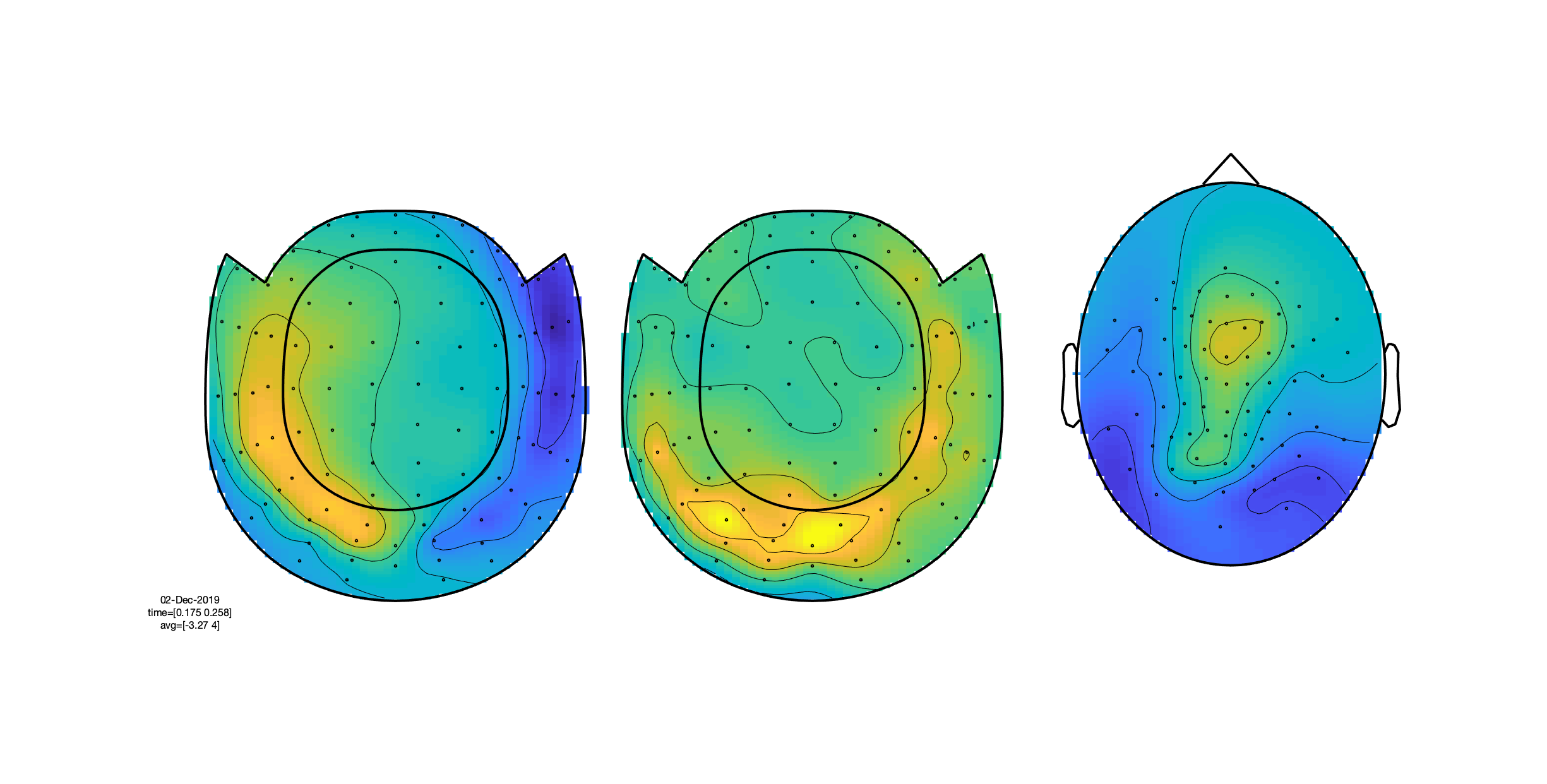
Figure: Topographies of average across selected latency window for one of the conditions.