Implementation of realistic electrode properties in forward volume conduction models

Description

In applications like epilepsy and brain-computer interface, electrocorticography electrode grids are often implanted in patients to detect normal and abnormal brain activity. For both applications, there is the need for assessing the sensitivity of current or newly-designed ECoG grids, whether the sensitivity could be improved, and how to eventually optimize the grid. These investigations can be conducted numerically, with adequate and adapted volume conduction models.

Commonly, in such models, electrodes are considered to record the potential in just a single point. However, we have shown the importance of explicitly including electrode properties in volume conduction models for accurately interpreting ECoG measurements. To achieve this type of simulation, the Finite Element Method for useful neuroscience simulations (FEMfuns) was developed, which allows knowledgeable neuroscientists to solve the forward problem in a variety of different geometrical domains, including various types of source models and electrode properties, such as resistive and capacitive materials, and the double layer that exists at the electrode-tissue interface. Here, as part of the project Into the Brain, we will incorporate FEMfuns into FieldTrip.

Organization of FEMfuns in FieldTrip

FEMfuns is a python based open-source pipeline and will be called externally from FieldTrip. Within FieldTrip, the headmodel and electrode positions are created, after which the forward solution is found using FEMfuns code under the hood. We split incorporating FEMfuns into FieldTrip in three steps:

• integrate complex meshing routines in FieldTrip
• test on sphere: compute the forward solutions in FieldTrip using a compiled binary of FEMfuns
• test on real dataset: compute forward solution in a realistically shaped head model (test the interaction of forward solutions computed with FEMfuns and pre-processing/source analysis routines implemented in FieldTrip)

The general workflow consists of calling many toolboxes and subroutines from MATLAB (see Figure 1).

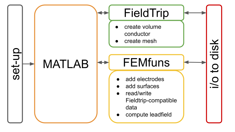
Figure1: Schematic representation of the general workflow.

The user is suggested to work from a MATLAB script, where they will call both FieldTrip and FEMfuns (see Figure 1). Before starting with such a script, it is necessary to set up both FieldTrip and FEMfuns (Figure 1, gray box).

While FieldTrip is MATLAB-based, FEMfuns is Python-based and, in particular, it externally calls Fenics to solve partial differential equations. For this, the whole procedure resembles a Russian doll (see Figure 2).

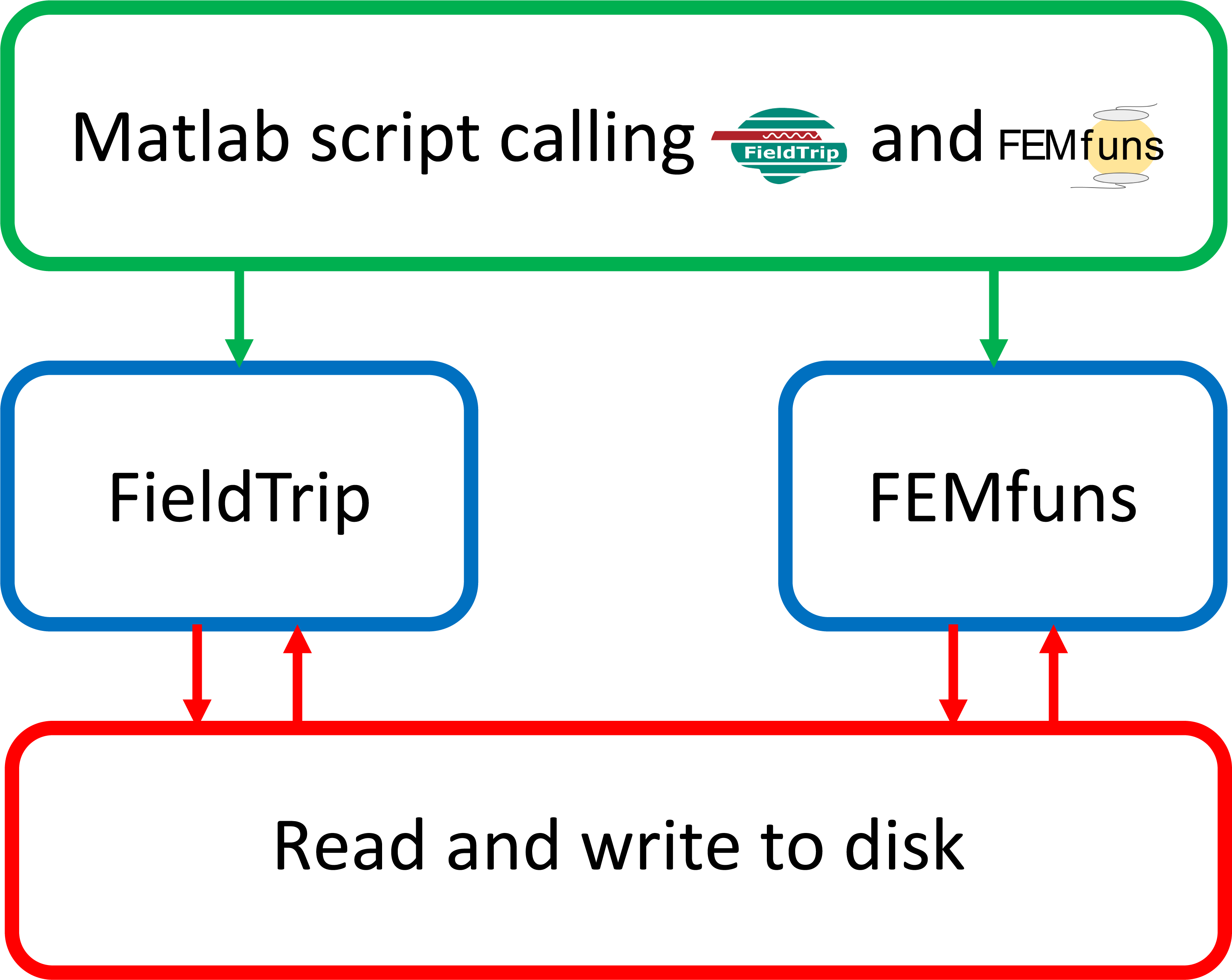
Figure 2: General workflow of the interface between FEMfuns and FieldTrip. From left to right: FieldTrip is called directly by MATLAB. To call FEMfuns from MATLAB, a shell script is launched in MATLAB. This shell script runs under the hood and calls FEMfuns routines implemented in Python.

Currently (April 2022), the MATLAB functions to add electrodes to an existing finite element head model and use leadfields computed in FEMfuns in FieldTrip analysis are available here

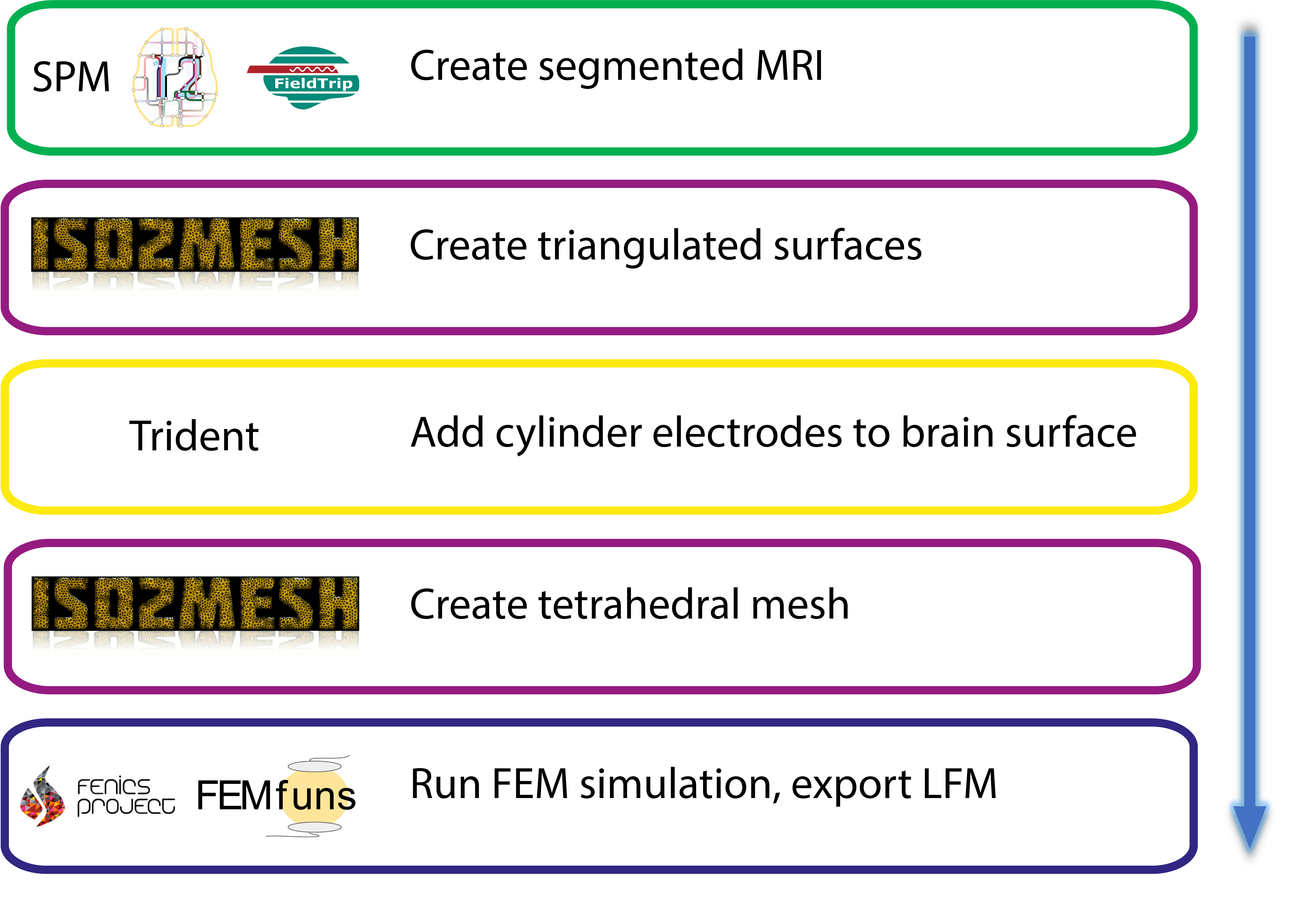
Besides FieldTrip, other external software is used in the workflow, e.g., FEniCS, Trident and ISO2MESH. A summary can be found in the schema below, which shows the order in which the softwares are used and for which steps in the pipeline:

Running a simulation with FieldTrip and FEMfuns combined

The following section illustrates an example where the FEMfuns pipeline is embedded in FieldTrip. The geometry, electrodes and sourcemodel are created in FieldTrip. These are used in FEMfuns to calculate leadfields by means of FEM with optional properties such as an electrode surface conductance and stimulating electrodes. Here, we present examples both in a simple sphere model and an MRI-based realistic head model.

Setting-up

The instructions to set up FEMfuns can be found on the Github page. Setting up is achieved in three steps:

Step 1: Download Anaconda: https://docs.continuum.io/anaconda/install/

wget https://repo.anaconda.com/archive/Anaconda3-2021.05-Linux-x86_64.sh
bash ./Anaconda3-2021.05-Linux-x86_64.sh

Step 2: Clone FEMfuns

git clone https://github.com/Donders-Institute/FEMfuns.git OR

wget https://github.com/Donders-Institute/FEMfuns/archive/refs/heads/master.zip

Step 3: Set-up the environment

Move to the cloned FEMfuns directory and create the conda environment.

cd FEMfunsDir
conda env create -f environment.yml
conda activate femfuns
conda develop pipeline_code/

Creating the environment is only needed once, but every new session where FEMfuns is needed the environment needs to be activated using

conda activate femfuns

Before starting with FieldTrip, it is important that you set up your MATLAB path properly.

cd <path_to_fieldtrip>
ft_defaults

Simulation

Two-sphere model

Then surfaces of two spheres can be created using FieldTrip:

% Create a spherical volume conductor with two spheres of radius 7 and 10 cm at the origin
csvol.o = [0, 0,0];
csvol.r = [7 10];
cfg = [];
cfg.numvertices = 1000;
csbnd = ft_prepare_mesh(cfg, csvol);

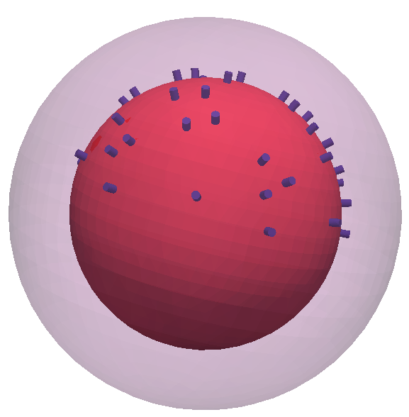
Realistic intracranial electrode surfaces are added to the inner sphere (representing the brain) at a few locations on the top half of the sphere.

%pick a few electrode positions on top of the sphere
sel = find(csbnd(1).pos(:,3)>0); sel = sel(1:100:end);
elec = [];
elec.elecpos = csbnd(1).pos(sel,:);
for i=1:length(sel)
  elec.label{i} = sprintf('elec%d', i);
end
elec.unit = 'cm';
% update the electrode sets to the latest standards
elec = ft_datatype_sens(elec);

% combine the brain surface with electrode surfaces and get inner points of the electrodes (here 'elecmarkers')
dp_elec = 0.5; %height  of the electrode cylinder
rad_elec = 0.2; %radius of the electrode cylinder
 [dented_elsurf,elecmarkers] = add_electrodes(csbnd(1), elec.elecpos, rad_elec, dp_elec);
merged_surfs = add_surf(dented_elsurf,csbnd(2)); %combine with the scalp

%create volumetric tetrahedral mesh
 [tet_node,tet_elem] = s2m(merged_surfs.pos,merged_surfs.tri, 1, 1, 'tetgen', [point_in_surf(csbnd(1));point_in_surf(csbnd(2));elecmarkers]);
%label the electrode surfaces where they make contact with the brain
el_faces = label_surf(tet_elem, 3:7, 1);

Currently volumes and surfaces are not combined in FieldTrip mesh structures. This is a work in progress. For now, a FieldTrip mesh structure is created separately including both volume and surface information:

%Construct the FT mesh structure
mesh.unit = 'cm';
mesh.pos = tet_node;
mesh.tet = tet_elem(:,1:4);
mesh.tri = el_faces(:,1:3);
mesh.boundary = el_faces(:,4);
mesh.boundarylabel = elec.label;
mesh.tissue = tet_elem(:,5);
mesh.tissuelabel = [{'brain'}, {'skull'},elec.label(:)'];

Next the FieldTrip sourcemodel is created:

% construct a vol to create the FT sourcemodel
vol.pos = mesh.pos;
vol.tet = mesh.tet;
vol.tissue = mesh.tissue;
vol.tissuelabel = mesh.tissuelabel;
vol.unit = mesh.unit;
vol.type = 'simbio';

cfg                 = [];
cfg.resolution      = 5; %in mm
cfg.headmodel       = vol;
cfg.inwardshift     = 1; %shifts dipoles away from surfaces
sourcemodel         = ft_prepare_sourcemodel(cfg);

Finally, the geometry and parameters are used by FEMfuns externally and the resulting leadfield is imported back into MATLAB with femfuns_leadfield.

% conductivities for brain, scalp and metal electrodes are set
conductivities = [0.33 0.01 1e10 1e10 1e10 1e10 1e10];
lf_rec = femfuns_leadfield(mesh,conductivities,sourcemodel,elec);

disp(lf_rec)
      dim: [3 3 3]
      pos: [27x3 double]
     unit: 'cm'
   inside: [27x1 logical]
      cfg: [1x1 struct]
leadfield: {1x27 cell}
    label: {'elec1'  'elec2'  'elec3'  'elec4'  'elec5'}

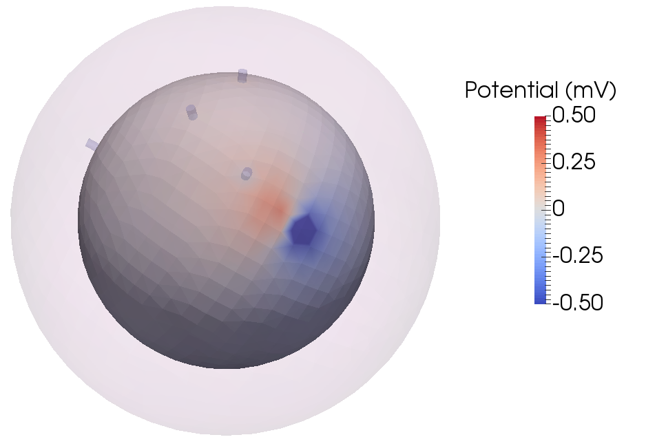
An example of the potential distribution on the inner sphere representing the brain (visualized using https://www.paraview.org/):

The structure of this leadfield grid can be used in FieldTrip, for example:

filename = fullfile(tempname, 'femfuns_leadfield');
ft_headmodel_interpolate(filename, elec, lf_rec, 'smooth', false);

Alternatively, stimulating electrodes can be used:

% Instead dipole sources, a stimulating and ground electrode is set.
% For boundary options, look for example here https://github.com/meronvermaas/FEMfuns/blob/master/separability/parameters_discelecins.py
sourcemodel.inside(:) = false;
elec.label{1} = ['stim_' elec.label{1}];
elec.label{2} = ['ground_' elec.label{2}];
mesh.boundarylabel = elec.label;
elec.params{1} = {1, 100, 'int'};
elec.params{2} = {0, 100, 'int'};
conductivities = [0.33 0.01 0 0 1e10 1e10 1e10];
lf_stim = femfuns_leadfield(mesh,conductivities,sourcemodel,elec);

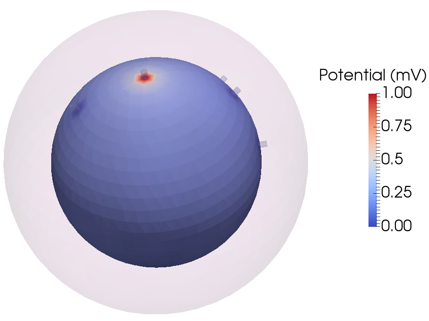
An example of the potential distribution on the inner sphere with the stimulating and ground electrode (visualized using https://www.paraview.org/):

The test script with all the above snippets put together is test_realistic_electrodes.m.

Realistic model of the head

The workflow for a realistic headmodel based on an anatomical MRI is comparable to the 2-sphere example. Here, we will go over the first steps where the mesh is created.

First, read in the mri data from FieldTrip (download the dataset here: Subject01.zip) and reslice it:

mri = ft_read_mri('Subject01.mri');
cfg     = [];
cfg.dim = mri.dim;
mri     = ft_volumereslice(cfg,mri);

Then, the anatomical mri is segmented in 3 non overlapping tissue types:

cfg           = [];
cfg.output    = {'brain','skull','scalp'};
segmentedmri  = ft_volumesegment(cfg, mri);

Next, triangulated surfaces can be created at the border of the tissues:

cfg        = [];
cfg.tissue={'brain','skull','scalp'};
cfg.numvertices = 3000;
cfg.method = 'iso2mesh';
bnd = ft_prepare_mesh(cfg,segmentedmri);

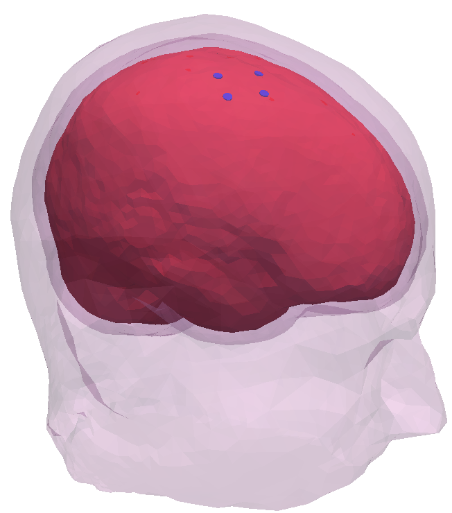
Now we are getting to the part of adding realistic electrodes. To do this, a FieldTrip electrode structure with 4 electrode positions on top of the brain is made:

el1 = [51.298 -26.242 106.026]; el2 = [38.926 -37.6445 105.965]; el3 = [31.47 -28.13 113.007]; el4 = [45.06 -13.467 112.423];
[~,I1] = min(abs(sum(bnd(1).pos-el1,2))); [~,I2] = min(abs(sum(bnd(1).pos-el2,2))); [~,I3] = min(abs(sum(bnd(1).pos-el3,2))); [~,I4] = min(abs(sum(bnd(1).pos-el4,2)));
sel = [I1 I2 I3 I4];
elec = [];
elec.elecpos = bnd(1).pos(sel,:);
for i=1:length(sel)
  elec.label{i} = sprintf('elec%d', i);
end
elec.unit = 'mm';
% update the electrode sets to the latest standards
elec = ft_datatype_sens(elec);

Then, we can combine the brain surface with electrode surfaces:

dp_elec = 0.5; %height  of the electrode cylinder
rad_elec = 2; %radius of the electrode cylinder
[dented_elsurf,elecmarkers] = add_electrodes(bnd(1), elec.elecpos, rad_elec, dp_elec);

% Add the skull and scalp to the brain again
merged_surfs = dented_elsurf;
for ii = 2:length(bnd)
    merged_surfs = add_surf(merged_surfs,bnd(ii));
end

Finally, we can create our volumetric tetrahedral mesh with 7 regions, 4 electrodes, brain, skull and scalp

[tet_node,tet_elem] = s2m(merged_surfs.pos,merged_surfs.tri, 1, 1, 'tetgen', [insidepoints; elecmarkers]);
%label the electrode surface where they make contact with the brain
el_faces = label_surf(tet_elem, length(bnd)+1:length(elec.elecpos)+length(bnd), 1);

The steps where the sourcemodel and leadfield is created is omitted here, since it consists of exactly the same steps as the 2-sphere example. The test script with the complete code is named test_headmodel_realistic_electrodes.m.

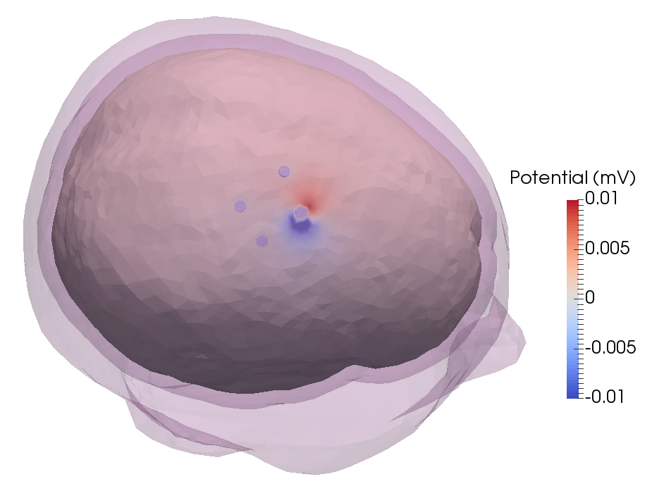
After running the code, an example of the potential distribution on the brain looks like (visualized using https://www.paraview.org/):

Disclaimer: as the number of cells increases, the RAM usage will quickly increase when converting the mesh to FEMfuns format and computing the FEM. In this realistic head model (with 7198480 tetrahedra) make sure to have at least 5GB available.

This work is supported by a grant from stichting IT projecten (StITPro).