Effects of tapering for power estimates
A simple way of looking at how (multi-)tapering affects the estimate of power in your signal is by using a very simple simulated signal. The ft_freqsimulation function allows you to quickly create a simulated signal with a well-defined frequency component in it. Subsequently you can use ft_freqanalysis with different taper settings to see the effect of tapering on your power estimate.
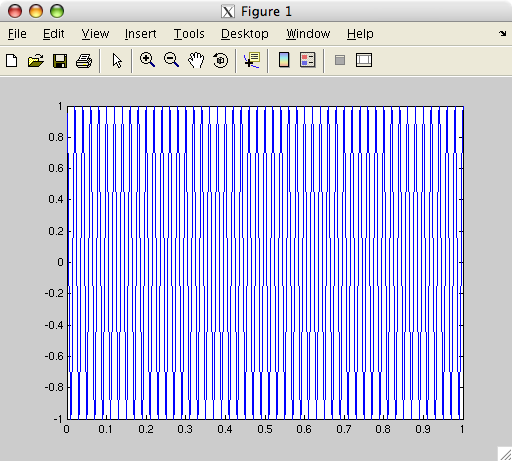
Create and plot a simulated signal. The simulated data contains only one trial, with a length of one second and a 50Hz sine wave.
clear all
close all

cfg = [];
cfg.method  = 'superimposed';
cfg.fsample = 1000;
cfg.numtrl  = 1;
cfg.trllen  = 1;
cfg.s1.freq = 50;
cfg.s1.ampl = 1;
cfg.s1.phase = 0;
cfg.noise.ampl = 0;
data = ft_freqsimulation(cfg);
figure
plot(data.time{1}, data.trial{1}(1,:))
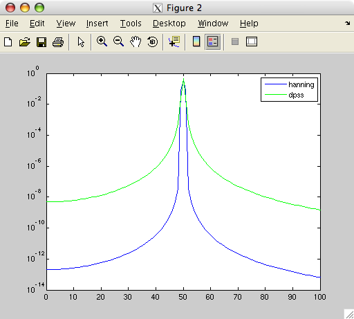
Compare the power estimate using a single Hanning taper with a single dpss taper (cfg.taper).
cfg        = [];
cfg.method = 'mtmfft';
cfg.output = 'pow';
cfg.pad    = 'maxperlen';
cfg.foilim = [0 100];
cfg.taper  = 'hanning';
freq       = ft_freqanalysis(cfg, data);
figure
semilogy(freq.freq, freq.powspctrm(1,:), 'b-');

cfg.taper     = 'dpss';
cfg.tapsmofrq = 1;   % i.e. no real smoothing
freq          = ft_freqanalysis(cfg, data);
hold on
semilogy(freq.freq, freq.powspctrm(1,:), 'g-');
legend({'hanning', 'dpss'});
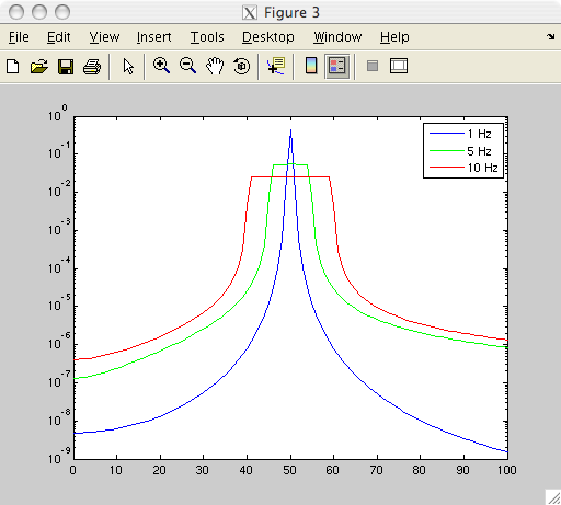
Look at the effect of multitapering with various amounts of smoothing (cfg.tapsmofrq).
cfg           = [];
cfg.method    = 'mtmfft';
cfg.output    = 'pow';
cfg.pad       = 'maxperlen';
cfg.foilim    = [0 100];
cfg.taper     = 'dpss';
cfg.tapsmofrq = 1;
freq          = ft_freqanalysis(cfg, data);
figure
semilogy(freq.freq, freq.powspctrm(1,:), 'b-');

cfg.tapsmofrq = 5;
freq          = ft_freqanalysis(cfg, data);
hold on
semilogy(freq.freq, freq.powspctrm(1,:), 'g-');

cfg.tapsmofrq = 10;
freq          = ft_freqanalysis(cfg, data);
hold on
semilogy(freq.freq, freq.powspctrm(1,:), 'r-');

legend({'1 Hz', '5 Hz', '10 Hz'});
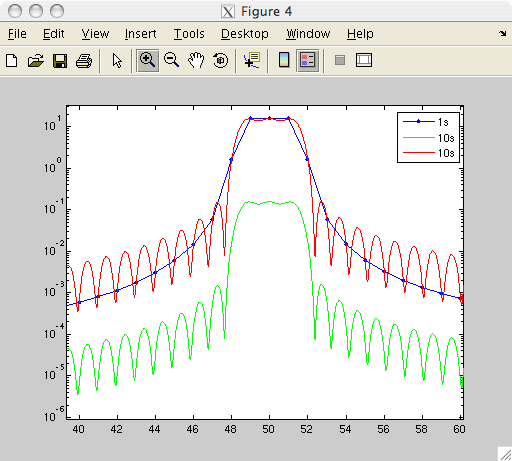
Look at the effect of spectral leakage of frequencies that are in between the natural frequencies of your time segment (cfg.pad). Note that the power spectral density per sqrt(Hz) decreases due to the zero-padding (compare the green and the blue). Multiplying the time series with a scaling factor fixes this, and makes the power spectral density estimates easier to compare (red and blue).
cfg           = [];
cfg.method    = 'mtmfft';
cfg.output    = 'pow';
cfg.foilim    = [0 100];
cfg.taper     = 'dpss';
cfg.tapsmofrq = 2;
cfg.pad       = 1;  % this is the same as the actual length of the data segment
freq          = ft_freqanalysis(cfg, data);
figure
semilogy(freq.freq, freq.powspctrm(1,:), 'b.-');

cfg.pad       = 100;
freq          = ft_freqanalysis(cfg, data);
hold on
semilogy(freq.freq, freq.powspctrm(1,:), 'g-');

data.trial{1} = data.trial{1}*10;           % equate the power spectral density to the first one
freq          = ft_freqanalysis(cfg, data);
hold on
semilogy(freq.freq, freq.powspctrm(1,:), 'r-');

legend({'1s', '5s', '10s'});