Perform modified Multiscale Entropy (mMSE) analysis on EEG/MEG/LFP data
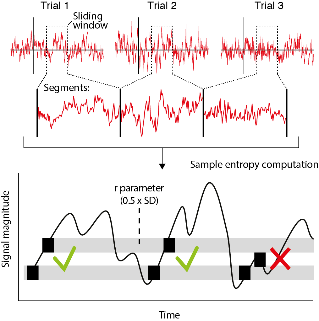
Recently, we have developed a novel algorithm based on multiscale entropy (Costa et al. 2002) called modified multiscale entropy (mMSE) that directly quantifies the temporal irregularity of time-domain EEG/MEG/LFP signals at longer and shorter timescales. In general, patterns of fluctuations in brain activity that tend to repeat over time are assigned lower entropy, whereas more irregular, non-repeating patterns yield higher entropy. To allow the investigation of dynamic changes in signal irregularity, we developed mMSE as a time-resolved variant, while also permitting assessment of entropy over atypically longer time scales by calculating across discontinuous, concatenated segments (Grandy et al.) (see the figure below).
Notably, mMSE is able to reveal brain-behavior links in EEG data that go undetected by conventional analysis methods such as spectral power, overall signal variation (SD), and event-related potentials (ERPs). Please see our preprints Kloosterman et al. and Kosciessa et al. for more information, and the tutorial folder on our Github page for a step-by-step explanation of the computation of mMSE within our fieldtrip MATLAB function.
Download and install the mMSE toolbox
To run entropy analysis on your data, download the mMSE toolbox for FieldTrip from our GitHub page as follows:
git clone https://github.com/LNDG/mMSE.git
or use the Download button on the GitHub page. The mMSE toolbox folder can be placed anywhere – it is not necessary to have it in your FieldTrip folder. However, the folder needs to be added to the path so MATLAB can find it. Furthermore, availability of the FieldTrip toolbox is required as the mMSE code relies on various FieldTrip helper functions. You can do this as follows:
addpath /path/to/your/mMSEfolder
After this step, you can call ft_entropyanalysis as any other FieldTrip function.
Run mMSE analysis on your data
ft_entropyanalysis takes as input preprocessed data as produced by ft_preprocessing. A few points are important to consider when preprocessing data for entropy analysis. First, it is advisable to apply a high-pass filter to your data to remove slow drifts. This is because entropy is computed by counting how often patterns reoccur in the time-domain data. To determine patterns, the data is first discretized by defining boundaries around each data point. These boundaries are set based on the standard deviation of the time-domain-signal. Slow drifts (e.g., due to electrode motion during the recording in EEG) will increase the standard deviation, thus loosening these boundaries, which in turn will result in more pattern matches and thus lower estimations of entropy (Kosciessa et al.). We have previously used a standard high-pass Butterworth filter during preprocessing, with a cutoff of 0.5 Hz on the continuous data (prior to defining trials) with good results.
Second, entropy is often computed for shorter and longer time scales. Longer time scales are accessed by increasingly coarsening the data by either averaging neighbouring data points or point skipping after low-pass filtering. Therefore, the timescales you can access depend on the sampling rate of the data. Given that entropy analysis can become computationally intensive with the high sampling rates and high number of channels typically used in E/MEG, we recommend downsampling to make the data easier to handle. In our example, we use a sampling rate of 256 Hz.
A final point pertains to the boundaries that are set around each data point to count pattern matches (see figure above). By increasingly smoothing the time series, coarse-graining affects not only on the signal’s entropy, but also its overall variation, as reflected in the decreasing standard deviation as a function of time scale (see Nikulin and Brismar, 2004). In the original implementation of the MSE calculation, the similarity parameter r was set as a proportion of the original (scale 1) time series’ standard deviation and applied to all the scales (Costa et al. 2002). Because of the decreasing variation in the time series due to coarse graining, the similarity parameter therefore becomes increasingly tolerant at longer time scales, resulting in more similar patterns and decreased entropy. This decreasing entropy can be attributed both to changes in signal complexity, but also in overall variation. To overcome this limitation, we advise recomputing the similarity parameter for each timescale, thereby normalizing MSE with respect to changes in overall time series variation at each scale. This feature can be controlled using the cfg.recompute_r parameter, as explained below.
To run mMSE analysis on your preprocessed data, first define the configuration:
cfg = [];
cfg.m                 = 2;                 % pattern length
cfg.r                 = 0.5;               % similarity parameter
cfg.timwin            = 0.5;               % sliding window size
cfg.toi               = -0.5:0.05:1;       % set this according to your trial length
cfg.timescales        = 1:42;              % timescale list
cfg.recompute_r       = 'perscale_toi_sp'; % when to recompute similarity parameter
cfg.coarsegrainmethod = 'filtskip';        % pointavg or filtskip
cfg.filtmethod        = 'lp';              % chooise low pass filter for pointskip
cfg.mem_available     = 16e9;              % memory available, in bytes
cfg.allowgpu          = true;              % allow GPU computations, if available
These settings define the following parameters in the computation:
cfg.mis the length of the data pattern that are being counted, consisting ofmandm+1patterns.cfg.m = 2means that 2-element patterns are counted and compared with the number of 3-element patterns.cfg.ris the pattern similarity parameter, indicating the proportion of the signal SD that is used for discretizing the data. A value of 0.5 indicates half the SD.cfg.timwinis the length of the sliding window used for selecting segments from the data.cfg.toiis a 1 x numtoi vector indicating the times on which the analysis windows (seecfg.timwin) should be centered (in seconds). The parameter is identical to thecfg.toiparameter in ft_freqanalysis.cfg.timescalesis a 1 x numscoi vector indicating the temporal scales for which entropy will be computed.cfg.timescalesis defined in scale numbers, in which scale 1 is the original time scale of the input data, corresponding to the sampling rate of the input data. For scale 2, the data is coarsegrained todata.fsample/2, for scale 3data.fsample/3, etc..cfg.recompute_rindicates in which stages of the analysis the r parameter should be recomputed.perscale_toi_spmeans the r parameter should be recomputed for each timescale, time point and starting point.cfg.coarsegrainmethodindicates the filtering procedure used to derive coarser (i.e., longer) time scales. It can either befilt_skip(default) (filter, then skip points; see Valencia et al., 2009) orpointavg(average groups of timepoints).cfg.filtmethodindicates the type of filter used in the ‘filt_skip’ method. It can either belp(default),hp,bp, ornofor no filtering.cfg.mem_availableindicates the memory available to perform computations (default 8e9 bytes). Entropy is computed in the function using 2-dimensional time-by-time matrices, which grow exponentially in size as the number of trials increases. If the matrices exceed this size, they are chunked and processed sequentially to avoid overloading memory.cfg.allowgpu1 (default) or 0 to indicate whether to allow computations to be run on a graphical processing unit (GPU), if available on the system. This can substantially speed up the computations. The function detects automatically both the presence of a MATLAB-compatible GPU, and the optimal chunk size depending on how much memory is available on the GPU.
After defining the cfg structure, entropy analysis is then simply run as follows:
[mmse] = ft_entropyanalysis(cfg, data);
The mmse output struct has the following fields:
mmse =
    dimord: 'chan_timescales_time'     defines how the numeric data should be interpreted
    sampen: [48x42x26 double]          sample entropy
     label: {48x1 cell}                the channel labels
timescales: [1x42 double]              the timescales, expressed in ms
   fsample: [1x42 double]              data sampling rate at each coarse graining step (timescale)
      time: [1x26 double]              the time, expressed in seconds
         r: [48x42x26 double]          the boundary similarity parameter computed for each bin
       cfg: [1x1 struct]               the configuration used by the function that generated this data structure
The mmse struct is structurally comparable to a freq structure as obtained from ft_freqanalysis, with the following exceptions: timescales replaces the frequency field, indicating the timescales axis; sampen replaces the powspctrm field, containing the resulting sample entropy values; fsample indicates the sampling rate of the data at each coarsegraining step; r contains the r values computed at each channel-by-timescales-by-time location.
If, after computing mMSE, you would like to use the FieldTrip functions for plotting, e.g., ft_multiplotTFR and computing statistics, i.e. ft_freqstatistics, the easiest way is to place the mMSE output into a freq structure (see ft_datatype_freq) so you can just plug the mMSE values into these functions.
Run standard MSE analysis on your data
Finally, it is also possible to run standard MSE analysis with our function. Standard MSE is computed across the complete timeseries at once so it has no time dimension. Furthermore, data is coarsened by averaging adjacent samples (point averaging). Finally, the r parameter is computed only once, instead of recomputed for each timescale. Please see the original MSE paper for details (Costa et al. 2002).
To run standard MSE analysis, define your cfg as follows:
cfg = [];
cfg.m                 = 2;                         % pattern length
cfg.r                 = 0.5;                       % similarity parameter
cfg.timwin            = data.time{1}(end)-data.time{1}(1);   % Assuming 1 trial with continuous data
cfg.toi               = median(data.time{1});      % middle time point
cfg.timescales        = 1:42;                      % timescale list
cfg.recompute_r       = 'per_toi';                 % use same similarity parameter across scales
cfg.coarsegrainmethod = 'pointavg';                % pointavg original implementation
cfg.mem_available     = 16e9;                      % memory available, in bytes
cfg.allowgpu          = true;                      % allow GPU computations, if available
[mse] = ft_entropyanalysis(cfg, data);
Please contact us via @neuro_klooster or kloosterman[at]mpib-berlin.mpg.de if you have questions or if you find bugs. You can also send us a Pull Request on the Github page.
This work was contributed by Niels Kloosterman, Julian Kosciessa, Liliana Polyanska, and Douglas Garrett within the Lifespan Neural Dynamics Group.
Please cite the following papers if you find the mMSE toolbox useful
Kloosterman NA, Kosciessa JQ, Lindenberger U, Fahrenfort JJ, Garrett DD. 2019. Boosting Brain Signal Variability Underlies Liberal Shifts in Decision Bias. Biorxiv 834614. doi:10.1101/834614
Kosciessa JQ, Kloosterman NA, Garrett DD. 2020. Standard multiscale entropy reflects neural dynamics at mismatched temporal scales: What’s signal irregularity got to do with it? Plos Comput Biol 16:e1007885. doi:10.1371/journal.pcbi.1007885
Grandy TH, Garrett DD, Schmiedek F, Werkle-Bergner M (2016) On the estimation of brain signal entropy from sparse neuroimaging data. Sci Rep 6:23073.