Using General Linear Modeling on time series data
For EEG and MEG analysis it is customary to use averaging to obtain ERPs/ERFs, whereas for fMRI it is customary to use GLMs. NIRS data falls a bit in between regarding the temporal characteristics of the acquisition system, which can be quite fast, and the characteristics of the physiological response, which is just as sluggish as the BOLD response. Consequently for NIRS data both averaging approaches are used (e.g., in the tutorials for single-channel and multi-channel NIRS data) and GLM approaches are used.
However, for the high temporal resolution EEG and MEG data it is also possible to use GLM approaches, as demonstrated for example in these papers:
- Convolution models for induced electromagnetic responses by Litvak et al.
- How much baseline correction do we need in ERP research? Extended GLM model can replace baseline correction while lifting its limits by Alday
- Regularization and a General Linear Model for Event-Related Potential Estimation by Kristensen et al.
- LIMO EEG: A Toolbox for Hierarchical LInear MOdeling of ElectroEncephaloGraphic Data by Pernet et al.
Since GLM is a very general and broadly applicable technique, it is not trivial to implement it in a single FieldTrip function. There are a number of functions that under the hood make use of GLMs, such as ft_regressconfound, ft_denoise_tsr, and various “statfuns” that have been used by researchers in combination with timelock-, freq- and sourcestatistics.
The following example demonstrates how you can use GLM in the analysis of time series data. It uses EEG data from a a study by Simanova et al. that investigated semantic processing of stimuli presented as pictures (black line drawings on white background), visually displayed text or as auditory presented words. The stimuli consisted of concepts from three semantic categories: two relevant categories (animals, tools) and a task category that varied across subjects, either clothing or vegetables. The same EEG dataset is also used elsewhere in the FieldTrip documentation and described in detail here. You can download the SubjectEEG.zip dataset from our download server.
General EEG preprocessing
The preprocessing of the EEG dataset is done largely similar as elsewhere on the website. Since we don’t want to segment the data in trials yet, and don’t use an explicit baselinecorrection, we apply a bandpass filter from 0.5 to 30 Hz.
cfg = [];
cfg.dataset     = 'subj2.vhdr';

cfg.bpfilter    = 'yes';
cfg.bpfreq      = [0.5 30];

cfg.reref       = 'yes';
cfg.channel     = {'all', '-64'};   % don't read the data from the electrode below the eye
cfg.implicitref = 'M1';             % the implicit (non-recorded) reference channel is added to the data
cfg.refchannel  = {'M1', '53'};     % the average of these will be the new reference, note that '53' corresponds to the right mastoid (M2)

data = ft_preprocessing(cfg);
We rename channel 53 (located at the right mastoid) to M2 for consistency.
chanindx = find(strcmp(data.label, '53'));
data.label{chanindx} = 'M2';
We also read the events from the original file, we need the timing to make the GLM.
event = ft_read_event(cfg.dataset);

% remove the New Segment
sel = strcmp({event.type}, 'Stimulus');
event = event(sel);

disp(unique({event.value}))
ans =
   1x41 cell array
   Columns 1 through 6
     {'S  1'}    {'S 12'}    {'S 13'}    {'S 21'}    {'S 27'}    {'S111'}
   Columns 7 through 12
     {'S112'}    {'S113'}    {'S121'}    {'S122'}    {'S123'}    {'S131'}
   Columns 13 through 18
     {'S132'}    {'S133'}    {'S141'}    {'S142'}    {'S143'}    {'S151'}
   Columns 19 through 24
     {'S152'}    {'S153'}    {'S161'}    {'S162'}    {'S163'}    {'S171'}
   Columns 25 through 30
     {'S172'}    {'S173'}    {'S181'}    {'S182'}    {'S183'}    {'S211'}
   Columns 31 through 36
     {'S212'}    {'S213'}    {'S221'}    {'S222'}    {'S223'}    {'S231'}
   Columns 37 through 41
     {'S232'}    {'S233'}    {'S241'}    {'S242'}    {'S243'}

% The trigger codes S112, S122, S132, S142 (animals) S152, S162, S172, S182 (tools)
% correspond to the presented visual stimuli. The trigger codes S113, S123, S133,
% S143 (animals) S153, S163, S173, S183 (tools) correspond to the presented auditory
% stimuli. These are the triggers we will select for now, allowing for some simple analyses.

trigVIS = {'S112', 'S122', 'S132', 'S142', 'S152', 'S162', 'S172', 'S182'};
trigAUD = {'S113', 'S123', 'S133', 'S143', 'S153', 'S163', 'S173', 'S183'};

sel = ismember({event.value}, trigVIS);
sampleVIS = [event(sel).sample];
sel = ismember({event.value}, trigAUD);
sampleAUD = [event(sel).sample];
There are 400 visual stimuli and 400 auditory stimuli. We can plot the time of each stimulus by converting the sample numbers into seconds.
figure
hold on
plot(sampleVIS./data.fsample, ones(size(sampleVIS)), 'rx')
plot(sampleAUD./data.fsample, ones(size(sampleAUD)), 'go')
xlabel('time (s)')
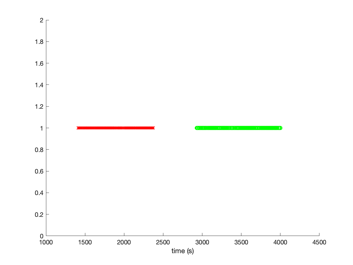
By inspecting the figure, we can learn multiple things: The visual and auditory stimuli are not randomized, but presented in a visual and in an auditory block. The whole experiment apparently lasted more than 4000 seconds, which is slightly more than an hour. Since we will process the data ac continuous time series, it is relevant to realize that there is also a lot of time in the recordings in which no interesting events happened.
cfg = [];
cfg.dataset             = 'subj2.vhdr';
cfg.trialdef.eventtype  = 'Stimulus';
cfg.trialfun = 'ft_trialfun_general';
cfg.trialdef.prestim    = 0.2;
cfg.trialdef.poststim   = 0.8;
cfg.trialdef.eventvalue = trigVIS;
cfg                     = ft_definetrial(cfg);

dataVIS = ft_redefinetrial(cfg, data);

cfg = [];
cfg.dataset             = 'subj2.vhdr';
cfg.trialdef.eventtype  = 'Stimulus';
cfg.trialfun = 'ft_trialfun_general';
cfg.trialdef.prestim    = 0.2;
cfg.trialdef.poststim   = 0.8;
cfg.trialdef.eventvalue = trigAUD;
cfg                     = ft_definetrial(cfg);

dataAUD = ft_redefinetrial(cfg, data);

cfg = [];
timelockVIS = ft_timelockanalysis(cfg, dataVIS);
timelockAUD = ft_timelockanalysis(cfg, dataAUD);
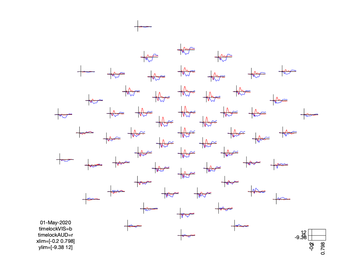
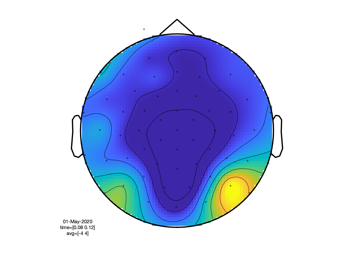
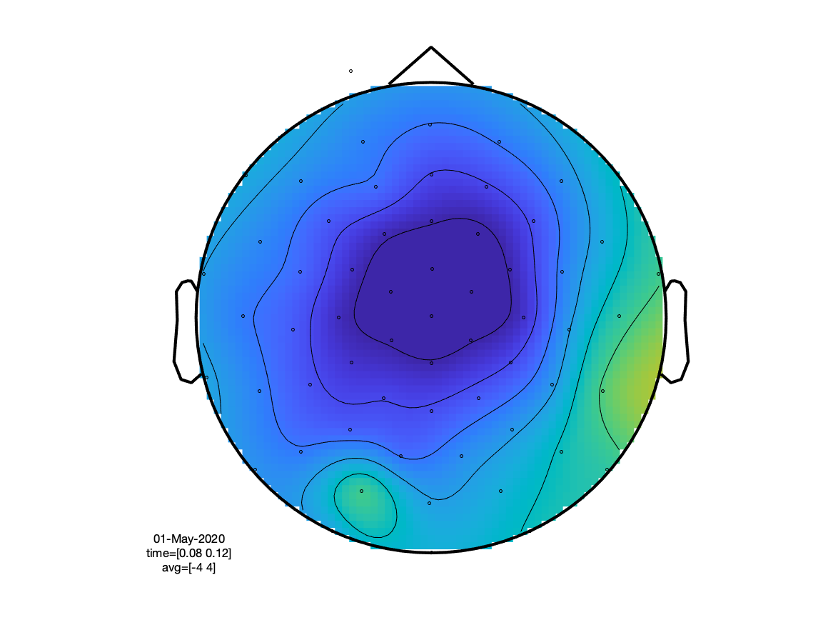
If we look at the sensory N100 component, we can see that (as expected) the visual condition has the extrema over the occipital cortex, whereas the auditory condition peaks at the vertex (due to the linked mastoids reference).
cfg = [];
cfg.layout      = 'easycapM10.mat';
cfg.baseline    =[-0.2 0];
ft_multiplotER(cfg, timelockVIS, timelockAUD)
cfg = [];
cfg.layout      = 'easycapM10.mat';
cfg.baseline    =[-0.2 0];
cfg.xlim        = [0.080 0.120];
ft_topoplotER(cfg, timelockVIS, timelockAUD)
Computing ERPs using a GLM
The ERPs are simply an average over all trials, which we can also compute using a GLM. To make it easier to relate to online tutorials on GLMs, we will use the convention that is common for fMRI data and follow the formulation from http://mriquestions.com/general-linear-model.html which explains GLMs in a very clear way.
We define the GLM model as
Y = X * B + err
where Y is data, X is the model, and B are the regression coefficients.
This means that the regression coefficients B can be estimated using the backslash or left division operation
Best = X\Y
which is similar to, but computationally more efficient as
Best = pinv(X)*Y
The estimated model data and residual can be estimated as
 Yest      = X * Best
 Yresidual = Y * Best
or when substituting the estimation for the regression coefficients
Yest      =     X * X\Y
Yresidual = Y - X * X\Y
The data Y has the time series of one channel (or voxel) in a column, which means that we have to transpose the data from the usual EEG representation. Let us first only consider a single channel. We will pick channel ‘1’, which corresponds to the vertex electrode. It should display a large AEP and a small VEP.
Y = data.trial{1}(1,:)';
The matrix X contains the model for the data. In ERP analysis we are averaging/modeling the EEG at each timepoint (relative to the onset of the trial) independently of all other timepoints. That means we need as many regressors as timepoints that we would consider in the trial. The trials that were selected for ft_timelockanalysis are one second and precisely 500 samples long. The model for a single trial therefore has 500 regressors and is simply constructed as
% Xtrial = eye(500);
Xtrial = speye(500);
Note that due to the large number of samples (about 2 million) and the large size of the model (500 columns), the matrix X is huge and the GLM estimation would take quite some time. But many of the entries in X are zero, and we can represent it as sparse matrix to make it memory efficient and speed up the computations.
This model repeats itself for each trial, and the total model for the whole continuous time series is constructed as follows. Rather than using the sample numbers from the event structure (see above), we are conveniently re-using the sampleinfo that is present in the segmented data structure. It contains two columns with the begin and end sample of each trial.
% X = zeros(length(Y), 500);
X = spalloc(length(Y), 500, 400*500);

for i=1:400
  begsample = dataAUD.sampleinfo(i,1);
  endsample = dataAUD.sampleinfo(i,2);
  X(begsample:endsample,:) = Xtrial;
end
We can estimate the regression coefficients with
Best      = X\Y;
Yest      = X * Best;
Yresidual = Y - X * Best;
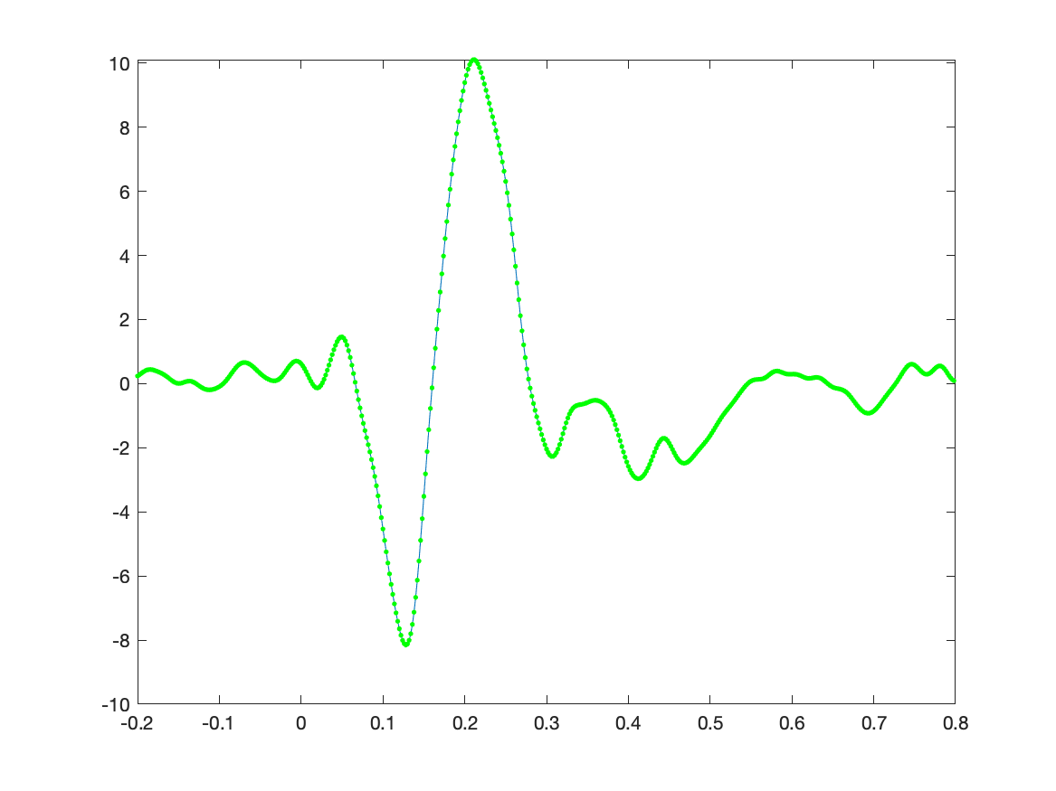
The ERP is now represented as the estimated regression coefficients and we can plot it with the following code. When we plot the original average on top of it, we see that they are the same.
figure
plot(timelockAUD.time, Best);
hold on
plot(timelockAUD.time, timelockAUD.avg(1,:), 'g.');
Computing ERPs in two conditions
We could now do the same thing as above for the visual condition separately, but we can also extend the model and estimate the regression coefficients at the same time. That means that we want to estimate the mean value at 1000 samples (500 for the auditory ERP, and 500 for the visual one). The model becomes
% X = zeros(length(Y), 2*500);
X = spalloc(length(Y), 2*500, 2*400*500);

% the first 500 columns represent the auditory average
for i=1:400
  begsample = dataAUD.sampleinfo(i,1);
  endsample = dataAUD.sampleinfo(i,2);
  X(begsample:endsample,1:500) = Xtrial;
end

% the second 500 columns represent the visual average
for i=1:400
  begsample = dataVIS.sampleinfo(i,1);
  endsample = dataVIS.sampleinfo(i,2);
  X(begsample:endsample,501:1000) = Xtrial;
end
In principle we can use the following code to plot the GLM design matrix. However, the number of elements (2 million times 1000) is too large to see much on a computer screen, which has way fewer pixels. If you zoom in on the right spot, you can recognize the design matrix, similar to how it is often displayed for example in SPM.
figure
imagesc(X)
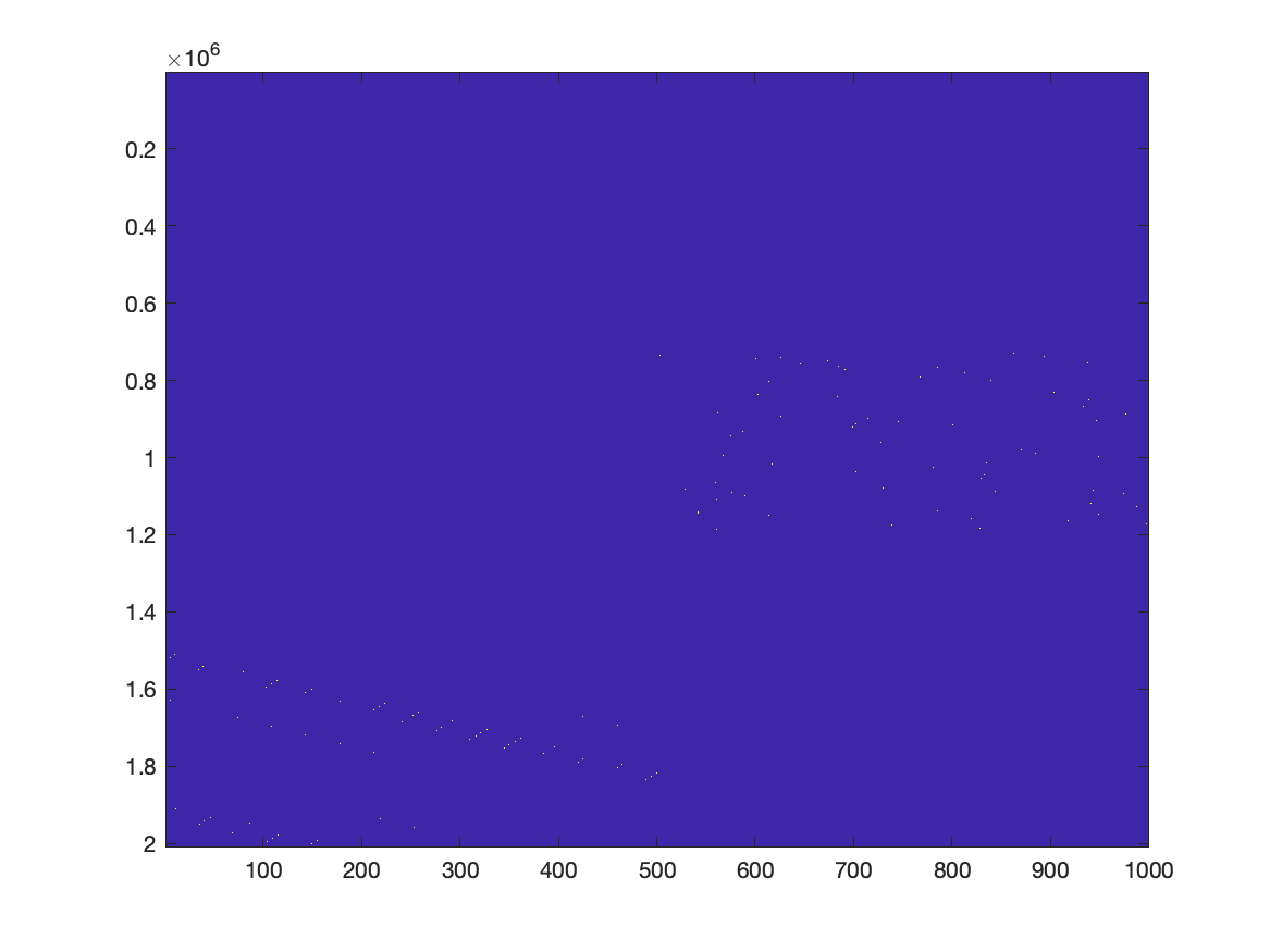
If we were to represent X as a normal matrix, it would be approximately 2e6 times 1000 times 8 bytes, corresponding to 16 GB of memory. By representing X as a sparse matrix, it not only makes the memory footprint much smaller, the computation is also much faster.
% X = sparse(X);   % not needed any more, it is directly constructed as a sparse matrix
Best = X\Y;
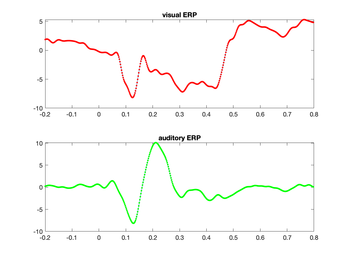
There are now 1000 estimated regression coefficients, which we can split in the ones for the auditory and the visual ERP.
Baud = Best(1:500);
Bvis = Best(501:1000);

figure
subplot(2,1,1)
plot(timelockVIS.time, Bvis);
hold on
plot(timelockVIS.time, timelockVIS.avg(1,:), 'r.');
title('visual ERP');

subplot(2,1,2)
plot(timelockAUD.time, Baud);
hold on
plot(timelockAUD.time, timelockAUD.avg(1,:), 'g.');
title('auditory ERP');
We can also look at how well the model explains the data
Yest      = X * Best;
Yresidual = Y - X * Best;

data_combined = [];
data_combined.time{1} = data.time{1};
data_combined.fsample = data.fsample;
data_combined.trial{1} = [
  Y'
  Yest'
  Yresidual'
  ];
data_combined.label = {
  'measured'
  'model'
  'residual'
  };

cfg = [];
cfg.viewmode = 'vertical';
cfg.blocksize = 10*60;          % show the data in pieces of 10 minutes
cfg.ylim = [-100 100];
cfg.mychan = {'model'};
cfg.mychanscale = 10;           % scale the model with a factor of 10x
ft_databrowser(cfg, data_combined);
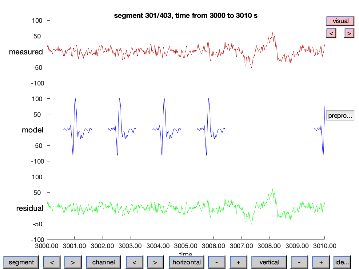
Note that in the visualization of the time series we are scaling the continuous representation of the model ERP potentials with a factor of 10. The averaged ERPs are of much smaller amplitude than the continuous EEG, and without scaling we could hardly recognize them.