How to incorporate head movements in MEG analysis
Description
Changes in head position during MEG sessions may cause a significant error in the source localization. Besides, the mixture of different head positions over time adds variance to the data that is not accounted for by the experimental manipulation. Thus head movements may deteriorate statistical sensitivity when analyzing MEG on both sensor and source levels. It is therefore recommended to incorporate head movements in the offline MEG analysis, see Stolk et al., NeuroImage 2013.
Continuous head localization information is stored in HLC channels (Head Localization Channels) in CTF MEG system. An example script here shows how to read these channels in FieldTrip and estimate the amount of movement offline. Information from these channels can also be used to track the head position in real time. You can download the TacStimRegressConfound.zip data used in this example script from our download server.
In general there are various ways that you can use the continuous head localization information.
- you can discard a subject or trial(s) from subsequent analysis if he/she moved too much
- you can regress out the movements from the processed data
- you can compensate the raw data for the movements
- you can correct the forward model (i.e. the leadfield) for the spatial blurring that is due to the movements
The first way of dealing with it requires that you visualize and decide on the movements. This is demonstrated in the first half of the example script.
The second way of dealing with the movements means that you perform ft_timelockanalysis, ft_freqanalysis or ft_sourceanalysis with the option cfg.keeptrials=yes. This will give trial estimates of the ERF, the power or the source strength for each trial. The effect that the variable head position has on those single-trial estimates can be estimated and removed from the data using ft_regressconfound. This method has been found to significantly improve statistical sensitivity following head movements, up to 30%, and is therefore demonstrated in the second half of the example script.
The third way of dealing with the movements requires that you make a spatial interpolation of the raw MEG data at each moment in time, in which you correct for the movements. In principle this could be done using the ft_megrealign function, but at this moment (May 2012) that function cannot yet deal with within-session movements.
The fourth way of dealing with the movements is implemented in the ft_headmovement function. It is not explained in further detail on this example page.
Reading-in and visualizing the head localization
Prepare configuration to define trials:
cfg                         = [];
cfg.dataset                 = 'TacStimRegressConfound.ds';
cfg.trialdef.eventtype      = 'UPPT001';
cfg.trialdef.eventvalue     = 4;
cfg.trialdef.prestim        = 0.2;
cfg.trialdef.poststim       = 0.3;
cfg.continuous              = 'yes';
cfg = ft_definetrial(cfg);
Read the data with the following HLC channels:
- HLC00n1 X coordinate relative to the dewar (in meters) of the nth head localization coil
- HLC00n2 Y coordinate relative to the dewar (in meters) of the nth head localization coil
- HLC00n3 Z coordinate relative to the dewar (in meters) of the nth head localization coil
    cfg.channel = {
      'HLC0011','HLC0012','HLC0013', ...
      'HLC0021','HLC0022','HLC0023', ...
      'HLC0031','HLC0032','HLC0033'
    };

    headpos = ft_preprocessing(cfg);
Determine the mean (per trial) circumcenter (the center of the circumscribed circle) of the three headcoils and its orientation (see subfunction at the bottom of this page)
% calculate the mean coil position per trial
ntrials = length(headpos.sampleinfo)
for t = 1:ntrials
  coil1(:,t) = [mean(headpos.trial{1,t}(1,:)); mean(headpos.trial{1,t}(2,:)); mean(headpos.trial{1,t}(3,:))];
  coil2(:,t) = [mean(headpos.trial{1,t}(4,:)); mean(headpos.trial{1,t}(5,:)); mean(headpos.trial{1,t}(6,:))];
  coil3(:,t) = [mean(headpos.trial{1,t}(7,:)); mean(headpos.trial{1,t}(8,:)); mean(headpos.trial{1,t}(9,:))];
end

% calculate the headposition and orientation per trial (for function see bottom page)
cc = circumcenter(coil1, coil2, coil3)
Now you can plot the head position relative to the first value, and compute the maximal position change.
cc_rel = [cc - repmat(cc(:,1),1,size(cc,2))]';

% plot translations
figure();
plot(cc_rel(:,1:3)*1000) % in mm

% plot rotations
figure();
plot(cc_rel(:,4:6))

maxposchange = max(abs(cc_rel(:,1:3)*1000)) % in mm
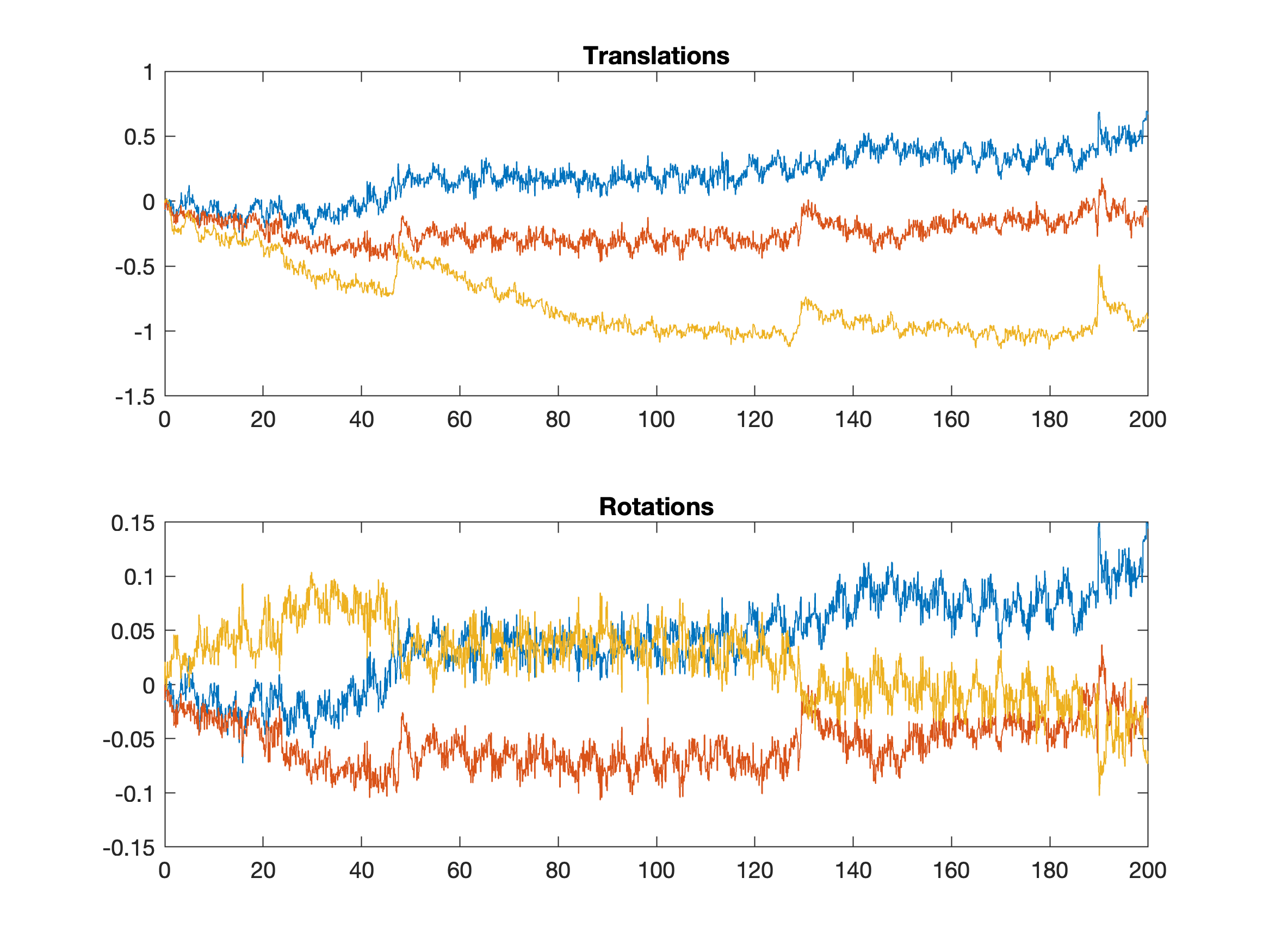
The figure illustrates head position changes during 1-hour MEG session (data used for this plot are different from those used in the example above). You may decide to exclude a subject from the subsequent analysis if the head movement exceeds a certain threshold.
Regressing out headposition confounds
MEG experiments typically involve repeated trials of an evoked or induced brain response. A mixture of different head positions over time adds variance to the data that is not accounted for by the experimental manipulation, thus potentially deteriorating statistical sensitivity. By using a general linear model, head movement related trial-by-trial variance can be removed from the data, both at the sensor- and source level. This procedure involves 3 step
- Preprocess the MEG data, for instance pertaining to an ERF analysis at the sensor level. Note the keeptrials = ‘yes’ when calling ft_timelockanalysis.
    % define trials
    cfg = [];
    cfg.dataset = 'TacStimRegressConfound.ds';
    cfg.trialdef.eventtype = 'UPPT001';
    cfg.trialdef.eventvalue = 4;
    cfg.trialdef.prestim = 0.2;
    cfg.trialdef.poststim = 0.3;
    cfg.continuous = 'yes';
    cfg = ft_definetrial(cfg);

   % preprocess the MEG data
   cfg.channel = {'MEG'};
   cfg.demean = 'yes';
   cfg.baselinewindow = [-0.2 0];
   cfg.dftfilter = 'yes'; % notch filter to filter out 50Hz
   data = ft_preprocessing(cfg);

   % timelock analysis
   cfg = [];
   cfg.keeptrials = 'yes';
   timelock = ft_timelockanalysis(cfg, data);
- Create trial-by-trial estimates of head movement. Here one may assume that the head is a rigid body that can be described by 6 parameters (3 translations and 3 rotations). The circumcenter function (see below) gives us these parameters. By demeaning, we obtain the deviations. In other words; translations and rotations relative to the average head position and orientation.
    % define trials
    cfg = [];
    cfg.dataset = 'TacStimRegressConfound.ds';
    cfg.trialdef.eventtype = 'UPPT001';
    cfg.trialdef.eventvalue = 4;
    cfg.trialdef.prestim = 0.2;
    cfg.trialdef.poststim = 0.3;
    cfg.continuous = 'yes';
    cfg = ft_definetrial(cfg);

    % preprocess the headposition data
    cfg.channel = {'HLC0011','HLC0012','HLC0013', ...
                   'HLC0021','HLC0022','HLC0023', ...
                   'HLC0031','HLC0032','HLC0033'};
    headpos = ft_preprocessing(cfg);

    % calculate the mean coil position per trial
    ntrials = length(headpos.sampleinfo)
    for t = 1:ntrials
      coil1(:,t) = [mean(headpos.trial{1,t}(1,:)); mean(headpos.trial{1,t}(2,:)); mean(headpos.trial{1,t}(3,:))];
      coil2(:,t) = [mean(headpos.trial{1,t}(4,:)); mean(headpos.trial{1,t}(5,:)); mean(headpos.trial{1,t}(6,:))];
      coil3(:,t) = [mean(headpos.trial{1,t}(7,:)); mean(headpos.trial{1,t}(8,:)); mean(headpos.trial{1,t}(9,:))];
     end

    % calculate the headposition and orientation per trial
    cc = circumcenter(coil1, coil2, coil3)

    % demean to obtain translations and rotations from the average position and orientation
    cc_dem = [cc - repmat(mean(cc,2),1,size(cc,2))]';
- Fit the headmovement regressors to the data and remove variance that can be explained by these confounds.
    % add head movements to the regressorlist. also add the constant (at the end; column 7)
    confound = [cc_dem ones(size(cc_dem,1),1)];

    % regress out headposition confounds
    cfg = [];
    cfg.confound = confound;
    cfg.reject = [1:6]; % keeping the constant (nr 7)
    regr = ft_regressconfound(cfg, timelock);
Figure
Example statistical results in a single-subject (baseline vs. task activity contrasts). With ft_regressconfound, sensor-level statistical sensitivity was increased after tactile stimulation (40-50 ms; note the more extreme t-scores in the upper panel). In a similar vein, source-level statistical sensitivity was increased after visual stimulation (0-500 ms; 65Hz; lower panel).
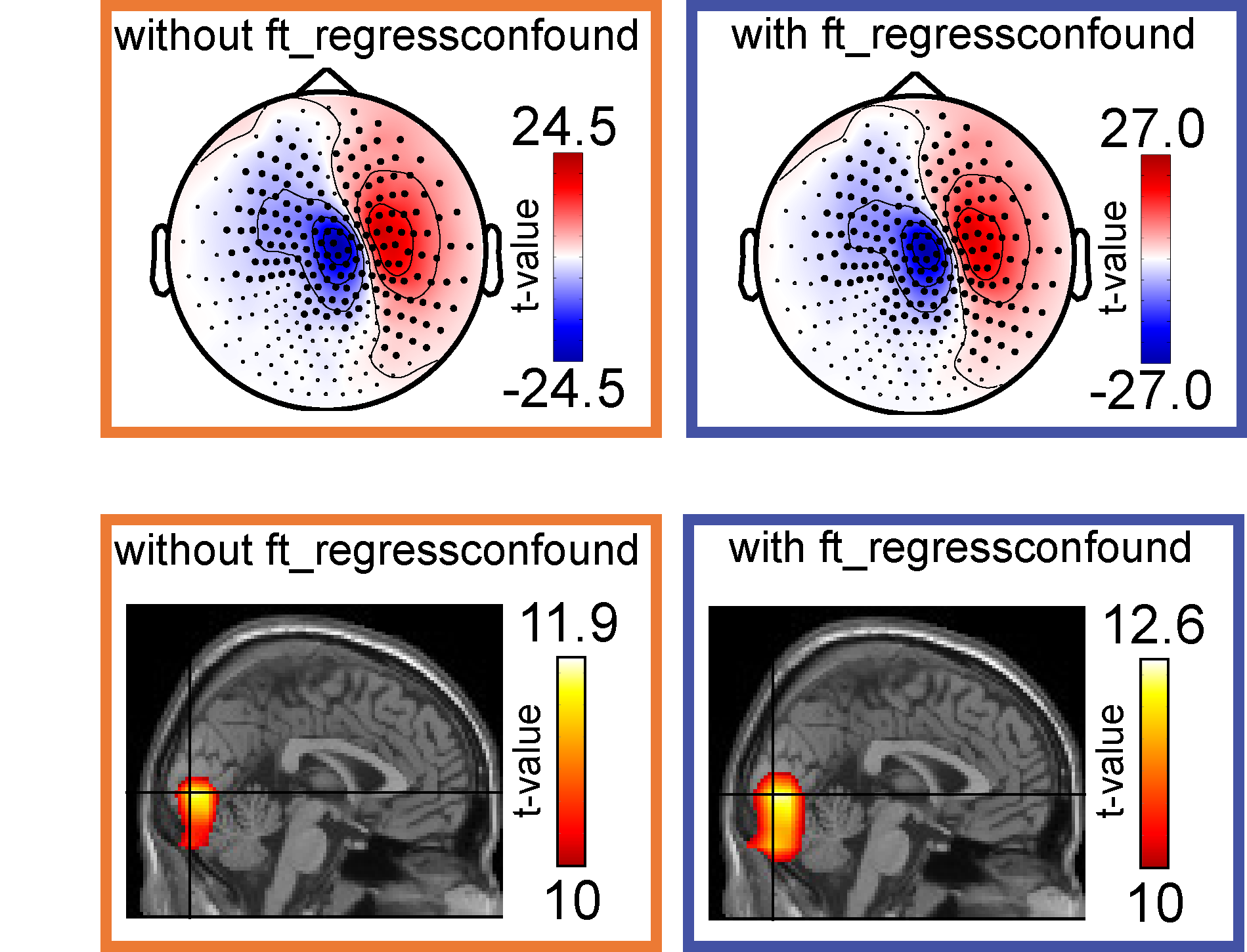
Figure taken from Stolk et al., NeuroImage 2013.
Practical issues
Some features of this GLM-based compensation method need emphasizing. These points are described in more detail in the ‘Testing the offline GLM-based head movement compensation’ section of Stolk et al., NeuroImage 2013.
First, ft_regressconfound can be applied to timelock, freq, and source data. The estimation of regression coefficients (beta weights of the head position data) is performed separately for each channel and each latency, in the case of timelock data. Consequently, after compensation, the sensor level data cannot be used anymore for source modeling. To employ the GLM based compensation on the source level, single trial estimates for the cortical locations of interest have to be made from the original sensor level data, preferably using a common spatial filter based on all trials. The beta weights are subsequently estimated for each cortical location and the variance in source amplitude over trials that is explained by the head movement is removed. It is therefore recommended to use ft_regressconfound as a final step prior to calling ft_timelockstatistics/ft_freqstatistics/ft_sourcestatistics.
Second, the same trials in the headposition data have to be selected as those present in the MEG data since these two will be fitted. And more or less related; this general linear modeling (GLM) approach only affects the signal variance and not the signal mean over trials (because the constant remains in the data). So when performing a group study, taking the subject mean to the group level statistics will not change these statistics. To benefit from improved statistical sensitivity after using ft_regressconfound, it is advised to take a measure that incorporates the consistency (over trials) of a neural effect to the group level. For instance, the t-descriptive, as obtained using an independent samples t-test on trials of one condition versus that of another. These t-values can then be tested at the group level for rejecting the null-hypothesis of no difference between conditions (T=0).
Finally, note that the circumcenter function is a helper function that calculates the position (geometrical center of the three localizer coils) and orientation of the head. This saves some degrees of freedom (df=6) as compared to taking into account the x,y,z-coordinates of each coil separately (n=3) as regressors (df=9). If you want to also use the squares, cubes, and derivatives as regressors (to account for non-linear effects of head motion on the MEG signal), this can save quite a bit of degrees. However, too large a number of covariates can reduce statistical efficiency for procedures. In that case, MATLAB will produce the Warning ‘Rank deficient’. A rule of thumb is to roughly have 10% of the sample size (based on chapter 8 of Tabachnick & Fidell (1996)).
Please cite this paper when you have used the offline head movement compensation in your study:
Stolk A, Todorovic A, Schoffelen JM, Oostenveld R. Online and offline tools for head movement compensation in MEG. Neuroimage. 2013 Mar;68:39-48. doi: 10.1016/j.neuroimage.2012.11.047.
Appendix: circumcenter
function [cc] = circumcenter(coil1,coil2,coil3)

% CIRCUMCENTER determines the position and orientation of the circumcenter
% of the three fiducial markers (MEG headposition coils).
%
% Input: X,y,z-coordinates of the 3 coils [3 X N],[3 X N],[3 X N] where N
% is timesamples/trials.
%
% Output: X,y,z-coordinates of the circumcenter [1-3 X N], and the
% orientations to the x,y,z-axes [4-6 X N].
%
% A. Stolk, 2012

% number of timesamples/trials
N = size(coil1,2);

%% x-, y-, and z-coordinates of the circumcenter
% use coordinates relative to point `a' of the triangle
xba = coil2(1,:) - coil1(1,:);
yba = coil2(2,:) - coil1(2,:);
zba = coil2(3,:) - coil1(3,:);
xca = coil3(1,:) - coil1(1,:);
yca = coil3(2,:) - coil1(2,:);
zca = coil3(3,:) - coil1(3,:);

% squares of lengths of the edges incident to `a'
balength = xba .* xba + yba .* yba + zba .* zba;
calength = xca .* xca + yca .* yca + zca .* zca;

% cross product of these edges
xcrossbc = yba .* zca - yca .* zba;
ycrossbc = zba .* xca - zca .* xba;
zcrossbc = xba .* yca - xca .* yba;

% calculate the denominator of the formulae
denominator = 0.5 ./ (xcrossbc .* xcrossbc + ycrossbc .* ycrossbc + zcrossbc .* zcrossbc);

% calculate offset (from `a') of circumcenter
xcirca = ((balength .* yca - calength .* yba) .* zcrossbc - (balength .* zca - calength .* zba) .* ycrossbc) .* denominator;
ycirca = ((balength .* zca - calength .* zba) .* xcrossbc - (balength .* xca - calength .* xba) .* zcrossbc) .* denominator;
zcirca = ((balength .* xca - calength .* xba) .* ycrossbc - (balength .* yca - calength .* yba) .* xcrossbc) .* denominator;

cc(1,:) = xcirca + coil1(1,:);
cc(2,:) = ycirca + coil1(2,:);
cc(3,:) = zcirca + coil1(3,:);

%% orientation of the circumcenter with respect to the x-, y-, and z-axis
% coordinates
v = [cc(1,:)', cc(2,:)', cc(3,:)'];
vx = [zeros(1,N)', cc(2,:)', cc(3,:)']; % on the x-axis
vy = [cc(1,:)', zeros(1,N)', cc(3,:)']; % on the y-axis
vz = [cc(1,:)', cc(2,:)', zeros(1,N)']; % on the z-axis

for j = 1:N
  % find the angles of two vectors opposing the axes
  thetax(j) = acos(dot(v(j,:),vx(j,:))/(norm(v(j,:))*norm(vx(j,:))));
  thetay(j) = acos(dot(v(j,:),vy(j,:))/(norm(v(j,:))*norm(vy(j,:))));
  thetaz(j) = acos(dot(v(j,:),vz(j,:))/(norm(v(j,:))*norm(vz(j,:))));

  % convert to degrees
  cc(4,j) = (thetax(j) * (180/pi));
  cc(5,j) = (thetay(j) * (180/pi));
  cc(6,j) = (thetaz(j) * (180/pi));
end