Independent component analysis (ICA) to remove ECG artifacts
Description
This script demonstrates how you can use ICA for cleaning the ECG artifacts from your MEG data. It consists of four steps:
- preparing the data for running an ICA
- ICA decomposition of the data
- identifying the components that reflect heart artifacts
- removing those components and backprojecting the data
Example dataset
You can run the code below on your own data. Alternatively, try with the ArtifactRemoval.zip example MEG dataset. This 275-channel CTF MEG dataset was acquired continuously with trials of 10 seconds. The subject was performing an experimental task, but that is not of relevance for this example. The CTF dataset is organized in trials of 10 seconds; as there are no discontinuities between trials, we can treat it as a continuous recording.
To load this dataset into MATLAB and preprocess with FieldTrip, use:
cfg                    = [];
cfg.dataset            = 'ArtifactRemoval.ds';
cfg.trialdef.eventtype = 'trial';
cfg = ft_definetrial(cfg);
It is important to remove all atypical artifacts (including SQUID jumps and muscle artifacts) prior to running your ICA, otherwise they may change the results you get. To remove artifacts on the example dataset, use:
cfg = ft_artifact_jump(cfg);
cfg = ft_rejectartifact(cfg);
cfg.trl([3 11 23],:) = []; % quick removal of trials with muscle artifacts, works only for this dataset!
You can now preprocess the data:
cfg.channel            = {'MEG', 'EEG058'}; % channel 'EEG058' contains the ECG recording
cfg.continuous         = 'yes';
data = ft_preprocessing(cfg);

% split the ECG and MEG datasets, since ICA will be performed on MEG data but not on ECG channel
% 1 - ECG dataset
cfg              = [];
cfg.channel      = {'EEG058'};
ecg              = ft_selectdata(cfg, data);
ecg.label{1}     = 'ECG'; % for clarity and consistency rename the label of the ECG channel
% 2 - MEG dataset
cfg              = [];
cfg.channel      = {'MEG'};
data_orig        = ft_selectdata(cfg, data);
Finally, you should downsample your data before continuing, otherwise ICA decomposition will take too long.
cfg            = [];
cfg.resamplefs = 150;
cfg.detrend    = 'no';
data           = ft_resampledata(cfg, data_orig);
Code
This script demonstrates how you can use ICA for cleaning the ECG artifacts from your MEG data. It starts by first doing a decomposition of the MEG data in the data segments of interest (i.e. the real trials in your experiment). Subsequently goes back to the original raw datafile and it reads the data segments around the QRS peaks that can easily be detected in the ECG channel. It uses the decomposition from the original data to estimate the timecourse of the components around the ECG artifacts. By looking at the component time courses (averaged), the coherence between the components and the ECG channel, and the spatial topographies, it is possible to determine which components are responsible for the ECG artifact in the MEG channels. Those components can then be removed from the original data.
cfg            = [];
cfg.method     = 'runica';
comp           = ft_componentanalysis(cfg, data);
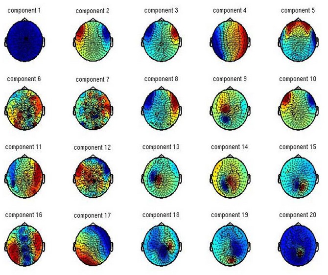
Once your component analysis is done, you can look at the topography of the components. Normally you will get the ECG components within the first 20 because the heartbeat is a very regular and very salient signal. You can almost always expect to get two ECG components, and they should look similar to each other, but slightly rotated. In the example below, these are components 4 and 17. They may come out as different components if you run the analysis on the same dataset, but their topography should look the same.
cfg           = [];
cfg.component = [1:20];       % specify the component(s) that should be plotted
cfg.layout    = 'CTF275.lay'; % specify the layout file that should be used for plotting
cfg.comment   = 'no';
ft_topoplotIC(cfg, comp)
To be certain these are the ECG components, you can also look at their time courses. In the image below, components 4 and 17 show a regular signal, typical for the heartbeat. You can also flip through all the trials, to see if this regular signal continues throughout the recording. (Note: ft_componentbrowser is deprecated; please use ft_databrowser instead.)
cfg          = [];
cfg.channel  = [2:5 15:18]; % components to be plotted
cfg.viewmode = 'component';
cfg.layout   = 'CTF275.lay'; % specify the layout file that should be used for plotting
ft_databrowser(cfg, comp)
However, given that you measured the heartbeat on a separate channel, you can use this information to extract the two components of interest. Two possible ways of doing this is by using timelock data, and frequency data. You do not need to use both unless you are uncertain which components to remove.
% go back to the raw data on disk and detect the peaks in the ECG channel, i.e. the QRS-complex
cfg                       = [];
cfg.continuous            = 'yes';
cfg.artfctdef.ecg.pretim  = 0.25;
cfg.artfctdef.ecg.psttim  = 0.50-1/1200;
cfg.channel               = {'ECG'};
cfg.artfctdef.ecg.inspect = {'ECG'};
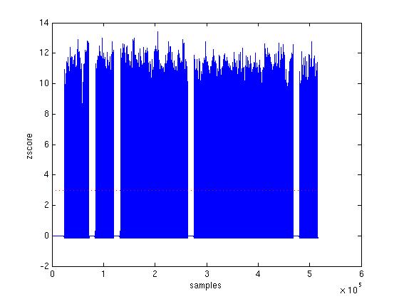
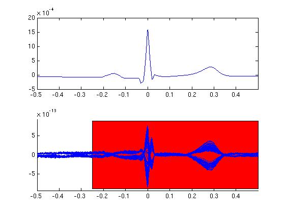
[cfg, artifact]           = ft_artifact_ecg(cfg, ecg);
You will be asked for feedback at two points while running this code. The visual display of your data should look similar to this. If it doesn’t, you may still have some jump artifacts in the data that you haven’t removed.
You can go on with the analysis now.
% preproces the data around the QRS-complex, i.e. read the segments of raw data containing the ECG artifact
cfg            = [];
cfg.continuous = 'yes';
cfg.padding    = 10;
cfg.dftfilter  = 'yes';
cfg.demean     = 'yes';
cfg.trl        = [artifact zeros(size(artifact,1),1)];
cfg.channel    = {'MEG'};
data_ecg       = ft_preprocessing(cfg, data_orig);

% resample to speed up the decomposition and frequency analysis, especially useful for 1200Hz MEG data
cfg            = [];
cfg.resamplefs = 300;
cfg.detrend    = 'no';
data_ecg       = ft_resampledata(cfg, data_ecg);
ecg            = ft_resampledata(cfg, ecg);

% decompose the ECG-locked datasegments into components, using the previously found (un)mixing matrix
cfg           = [];
cfg.unmixing  = comp.unmixing;
cfg.topolabel = comp.topolabel;
comp_ecg      = ft_componentanalysis(cfg, data_ecg);

% append the ecg channel to the data structure;
comp_ecg      = ft_appenddata([], ecg, comp_ecg);

% average the components timelocked to the QRS-complex
cfg           = [];
timelock      = ft_timelockanalysis(cfg, comp_ecg);
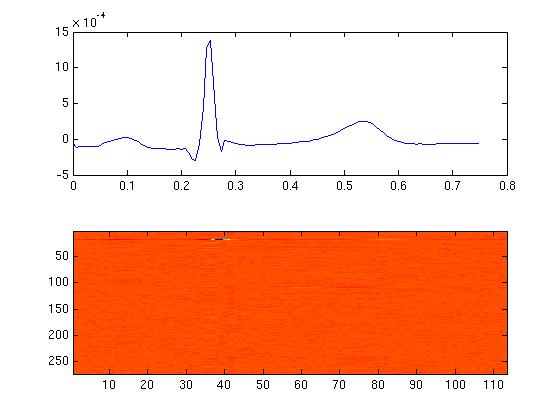
Below is the code for generating images which will help you detect which components correlate more with the time course of the heartbeat. Normally you will get two components that follow each other quickly in time. By zooming into the second subplot of the second graph you can see which numbers these components have. In this case it is indeed components 4 and 17.
% look at the timelocked/averaged components and compare them with the ECG
figure
subplot(2,1,1); plot(timelock.time, timelock.avg(1,:))
subplot(2,1,2); plot(timelock.time, timelock.avg(2:end,:))
figure
subplot(2,1,1); plot(timelock.time, timelock.avg(1,:))
subplot(2,1,2); imagesc(timelock.avg(2:end,:));
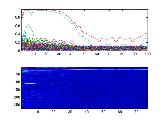
A second way of finding which components contain the ECG artifacts is through calculating coherence of your component analysis with the heartbeat. Two components should be prominent here as well.
% compute a frequency decomposition of all components and the ECG
cfg            = [];
cfg.method     = 'mtmfft';
cfg.output     = 'fourier';
cfg.foilim     = [0 100];
cfg.taper      = 'hanning';
cfg.pad        = 'maxperlen';
freq           = ft_freqanalysis(cfg, comp_ecg);

% compute coherence between all components and the ECG
cfg            = [];
cfg.channelcmb = {'all' 'ECG'};
cfg.jackknife  = 'no';
cfg.method     = 'coh';
fdcomp         = ft_connectivityanalysis(cfg, freq);

% look at the coherence spectrum between all components and the ECG
figure;
subplot(2,1,1); plot(fdcomp.freq, abs(fdcomp.cohspctrm));
subplot(2,1,2); imagesc(abs(fdcomp.cohspctrm));
Again, by zooming in to the lower subplot, you can see that in this case those are components 4 and 17.
Based on the figures, you now should select the components that explain the ECG artifact, and remove them from your data. The resulting dataset will contain the measured brain activity, with the variance attributable to the heartbeat partialled out.
% decompose the original data as it was prior to downsampling to 150Hz
cfg           = [];
cfg.unmixing  = comp.unmixing;
cfg.topolabel = comp.topolabel;
comp_orig     = ft_componentanalysis(cfg, data_orig);

% the original data can now be reconstructed, excluding those components
cfg           = [];
cfg.component = [4 17];
data_clean    = ft_rejectcomponent(cfg, comp_orig,data_orig);
