Using GLM to analyze NIRS timeseries data
This is an example MATLAB script that demonstrates how to compute a simple GLM on the fingertapping NIRS data that is also used in the tutorial on preprocessing and averaging of single-channel NIRS data. The data is available from our download server.
We start with reading the NIRS data from disk.
cfg = [];
cfg.dataset = 'motor_cortex.oxy3';
data_nirs = ft_preprocessing(cfg);
Construct a number of additional channels with the task/stimulus details
Then we read the events, which are represented as markers or triggers, indicating the samples in the data in which the fingertapping started or stopped. We use these to make some additional continuously represented channels that represent the onset, offset, and the motion. Furthermore, we can add two channels for a constant offset, and for a slope. These can be used to remove the baseline and a constant drift in the signal over time.
event = ft_read_event(cfg.dataset);

data_stim = [];
data_stim.time = data_nirs.time;
data_stim.label = {
  'onset'
  'offset'
  'motion'
  'constant'
  'slope'
  };
data_stim.chantype = repmat({'stimulus'}, size(data_stim.label));  % Homer stires the experimental design as stimulus (s)
data_stim.chanunit = repmat({'unknown'}, size(data_stim.label));

move_onset  = [event(strcmp({event.value}, 'A')).sample]; % this indicates the beginning of the movement
move_offset = [event(strcmp({event.value}, 'B')).sample]; % this indicates the end of the movement

nchans   = length(data_stim.label);
nsamples = length(data_stim.time{1}); % it is a continuous representation, hence one trial/segment

data_stim.trial{1} = zeros(nchans, nsamples);
data_stim.trial{1}(1,move_onset)  = 1;
data_stim.trial{1}(2,move_offset) = 1;
for i=1:numel(move_onset)
  data_stim.trial{1}(3,move_onset(i):move_offset(i)) = 1;
end
data_stim.trial{1}(4,:) = ones(1,nsamples);
data_stim.trial{1}(5,:) = linspace(0,1,nsamples);

% show the experimental design as a matrix
figure
imagesc(data_stim.trial{1})
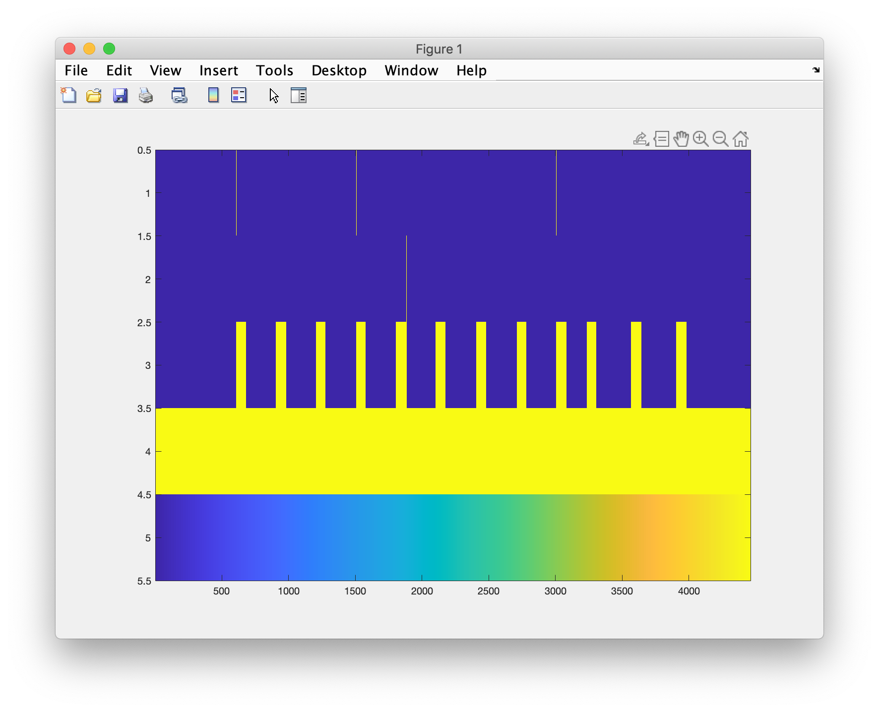
You actually have to zoom in a lot to see all details, since there are more samples than horizontal pixels on your screen
Combine the NIRS data and the description of the task/stimulus details
cfg = [];
data_combined = ft_appenddata(cfg, data_nirs, data_stim);

% also keep the optode structure, we need it further down for fieldtrip2homer and plotting
data_combined.opto = data_nirs.opto;
Perform a GLM analysis
This is explained on http://mri-q.com/general-linear-model.html with an excellent introduction, and on https://www.brainvoyager.com/bv/doc/UsersGuide/StatisticalAnalysis/TheGeneralLinearModel.html.
close all

% take the data from the FieldTrip data structures
y = cat(2, data_nirs.trial{:})';
x = cat(2, data_stim.trial{:})';
After further processing and artifact removal you could also take them from the data_combined structure, which would ensure that they keep nicely aligned - also when you discard artifact segments. But here we simply include all samples.
% use the default canonical haemodynamic response function (HRF) from SPM
ft_hastoolbox('spm12', 1);
h = spm_hrf(1/data_nirs.fsample);
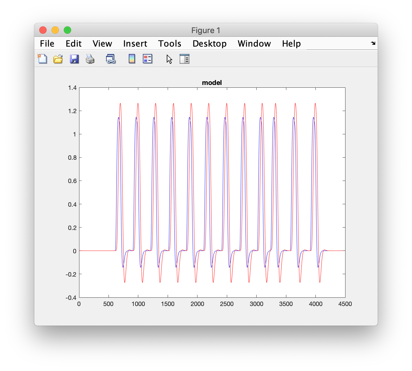
% plot the original regressor
figure
plot(x(:,3), 'b')
hold on
title('model')
% convolve the design with the HRF
xc = convn(x', h')';
xc = xc(1:nsamples,:); % remove the trailing part
% replace the first three columns of the design with the HRF convolved version
x(:,1:3) = xc(:,1:3);
% plot the HRF convolved regressor
plot(x(:,3), 'r-')
Remove the baseline, see also ft_preproc_baselinecorrect and ft_preproc_detrend. This is beneficial here, since the experimental regressors are not orthogonal to the confound regressors.
y = ft_preproc_polyremoval(y', 2)';
% fit the general linear model (GLM)
% y = x * b + e
b = x \ y;
model = x * b;
e = y - model;
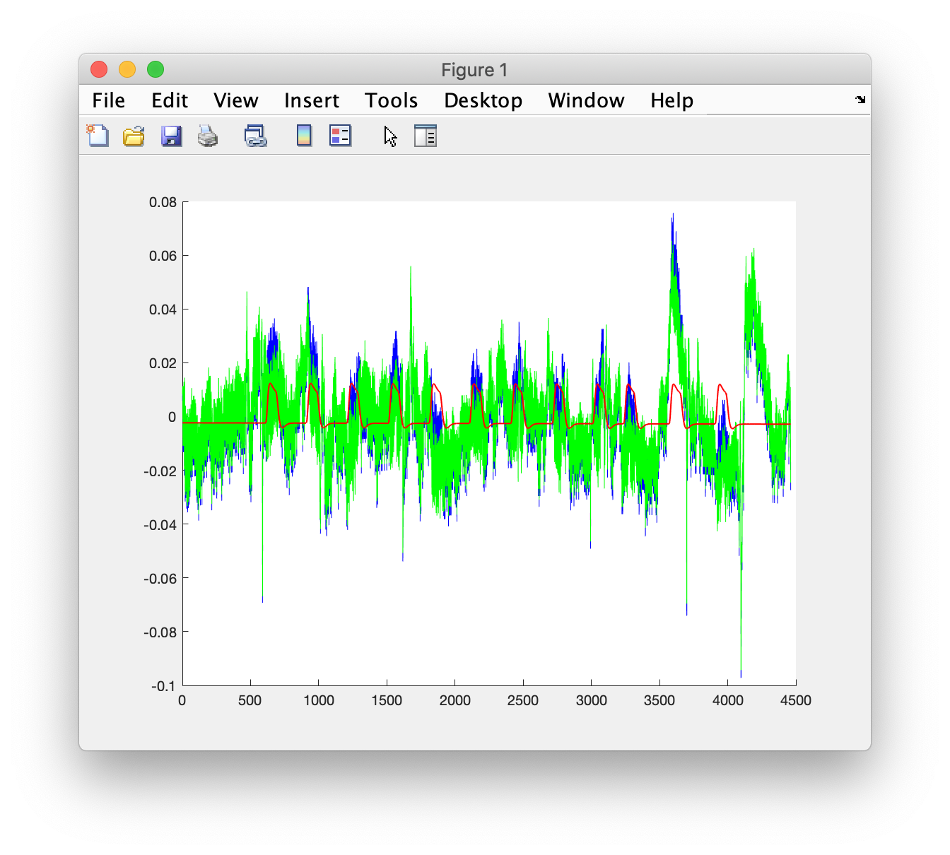
chan = find(strcmp(data_nirs.label, 'Rx4b-Tx5 [860nm]'));
figure
hold on
plot(y(:,chan), 'b')
plot(e(:,chan), 'g')
plot(model(:,chan), 'r')
set(h, 'LineWidth', 1)
legend({'data', 'noise', 'model'});
title('fit to data')
Convert the fitted model into statistical parameters
[n,p] = size(x);
r2 = var(model)./var(y);
f = r2*(n-p) ./ ((1-r2)*(p-1));
c = [0 0 1 0 0]';
t = (c' * b) ./ sqrt(var(e) * (c' * (x'*x) * c));
It would be possible to make topographic maps of these t-values.
Doing the same using the Homer data representation
We can also do this analysis using the Homer data representation. For that we can convert the data from FieldTrip to Homer
nirs = fieldtrip2homer(data_combined);
and then take the data matrix y and the experimental design matrix x
y = nirs.d;
x = nirs.s;
Subsequently we could continue as above …