documentation / example / source / phantom_topographies /
Plot the topographies of HPI coils and different MEG phantoms
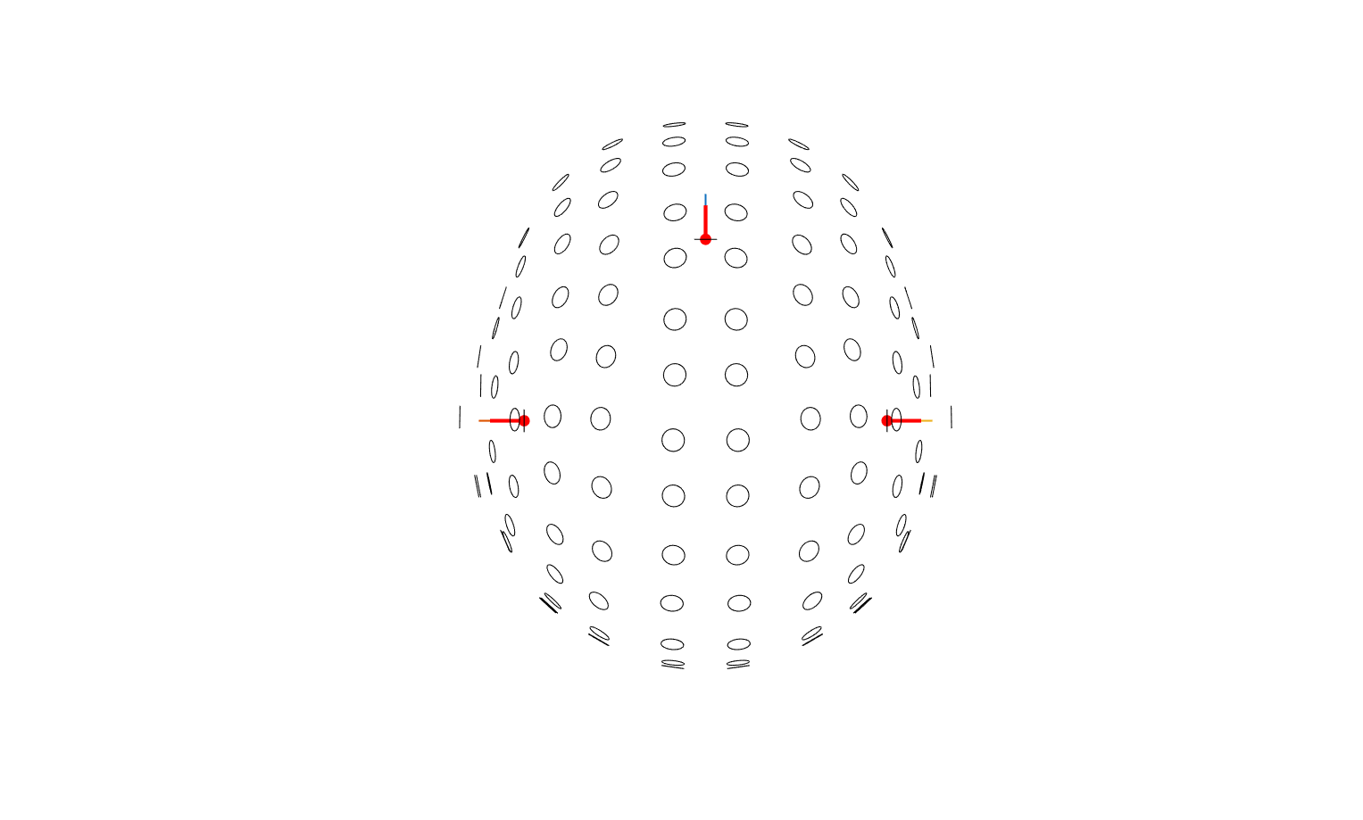
In this example we compute the spatial topographies of a variety of MEG phantoms: first for three magnetic dipole coils that are placed as head position indicators (HPIs) on the location of the nasion and left and right preauricular points (LPA and RPA). Subsequently, we compute and plot the topographies for different types of MEG phantoms.
All computations below are done for 144 radial OPM channels placed in a FieldLine beta 2 helmet, but they could equally well be done for any other arragmenent of the MEG sensors, either for SQUID or for OPM sensors. You can also provide your own sensor definition, see this FAQ and the documentation in the ft_datatype_sens function.
When changing the MEG sensor array to another template or to your own, please consider that the sensor arrays can be expressed relative to different head coordinaye systems. The FieldLine beta 2 helmet used below follows the Neuromag convention and has the x-axis towards the right, the y-asix to the front, and the z-axis in the superior direction.
% The following templates are located in fieldtrip/template/gradiometer

% load bti148.mat
% load bti248.mat
% load bti248grad.mat
% load ctf64.mat
% load ctf151.mat
% load ctf275.mat
% load neuromag122.mat
% load neuromag306.mat
% load yokogawa160.mat
% load yokogawa208.mat
% load fieldlinealpha1.mat

load fieldlinebeta2.mat
Since all phantoms that we will consider here for now are coils that emulate a magnetic dipole phantoms, we construct an infinite volume conductor.
headmodel = ft_headmodel_infinite();
headmodel.unit = 'm';
Construct the phantom coils
The snippets of code for the different HPI or phantom coil arrangements below are all handled in the same way. We first construct a phantom structure with the positions and orientations of the phantom coils. Those are formatted similar to the FieldTrip grad structure, so that we can use the ft_plot_sens function for visualization.
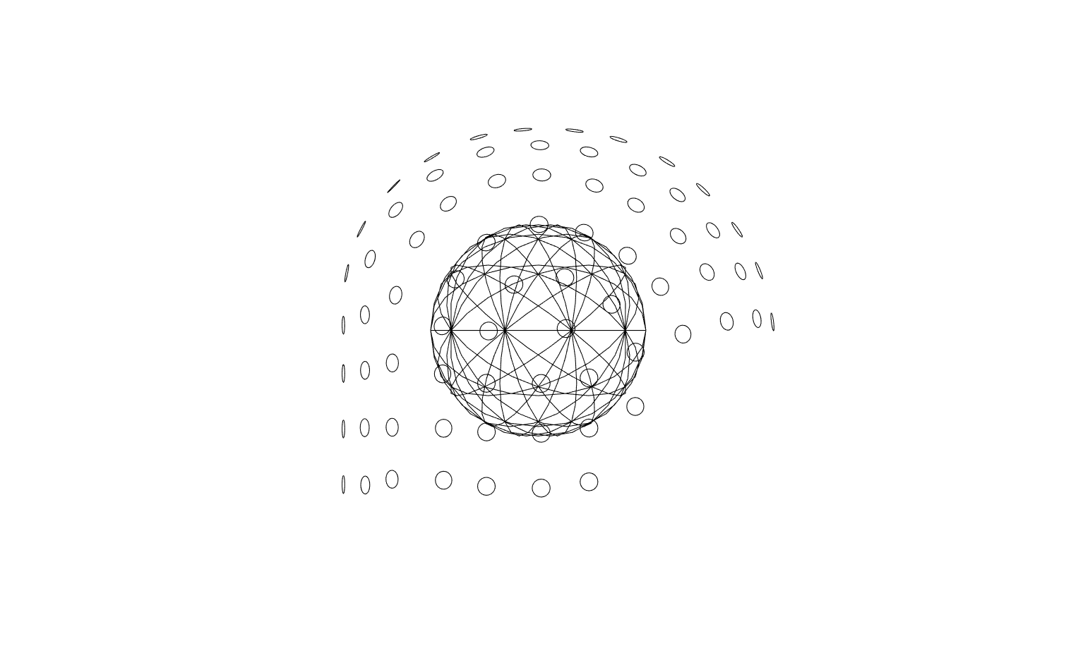
After constructing one of the phantom structures, we plot the phantom coils together with the OPM helmet and then we compute and visualise the spatial topographies of all the phantom coils.
To move or rotate either the OPM helmet or the phantom coil array, you can use ft_transform_geometry or other functions for realignment.
HPI coils on the anatomical landmarks
% this approximates where I would expect the nose and ears
nas = [0  8 0]/100;
lpa = [-8 0 0]/100;
rpa = [+8 0 0]/100;

phantom.coilpos = [
    nas
    lpa
    rpa
];
phantom.coilori = [
     0 1 0
    -1 0 0
    +1 0 0
];
phantom.label = {
    'nas'
    'lpa'
    'rpa'
};
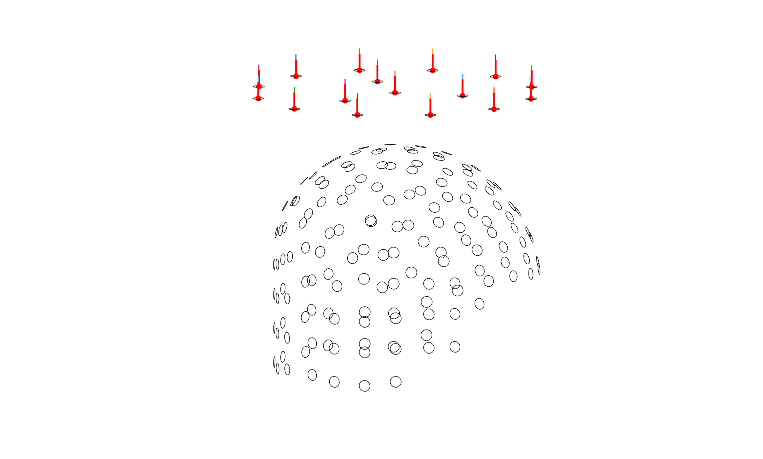
QuSpin HALO
QuSpin has designed their HALO to calibrate the OPM sensor positions and orientations. It consists of a circular printed circuit board (PCB) with 16 electromagnetic coil positions arranged in three distinct concentric layouts. Each of the 16 coils has a diameter of approximately 22 mm. The flat circular board is mounted on a base that holds it roughly 5 cm directly above the participant’s helmet or sensor array. It is described in the publication “Determining sensor geometry and gain in a wearable MEG system” by Hill et al. (2025).
% Outer Circle: 12 dipolar coils are evenly spaced every 30 degrees around a circle with a radius of 12.7 cm.
% Inner Circle: 3 dipolar coils are spaced at 120-degree intervals around a smaller circle with a radius of 6.3 cm.
% Center: 1 final dipole coil is positioned directly at the center of the circular board.

phantom.coilpos = zeros(16,3);
phantom.coilori = zeros(16,3);
phantom.coilori(:,3) = 1; % they are all pointing in the z-direction
% phantom.label = {'1', '2', '3', '4', '5', '6', '7', '8', '9', '10', '11', '12', '13', '14', '15', '16'};
phantom.label = {'12', '1', '2', '3', '4', '5', '6', '7', '8', '9', '10', '11', '13', '16', '15', '14'};

for i=1:12
    [x, y] = pol2cart(pi/2 - (i-1)*2*pi/12, 0.127);
    phantom.coilpos(i,1) = x;
    phantom.coilpos(i,2) = y;
    phantom.coilpos(i,3) = 0.05 + max(fieldlinebeta2.coilpos(:,3)); % 5 cm above the top of the helmet
end

for i=1:3
    [x, y] = pol2cart(pi/2 - (i-1)*2*pi/3, 0.063);
    phantom.coilpos(12+i,1) = x;
    phantom.coilpos(12+i,2) = y;
    phantom.coilpos(12+i,3) = 0.05 + max(fieldlinebeta2.coilpos(:,3)); % 5 cm above the top of the helmet
end

phantom.coilpos(16,1) = 0;
phantom.coilpos(16,2) = 0;
phantom.coilpos(16,3) = 0.05 + max(fieldlinebeta2.coilpos(:,3)); % 5 cm above the top of the helmet
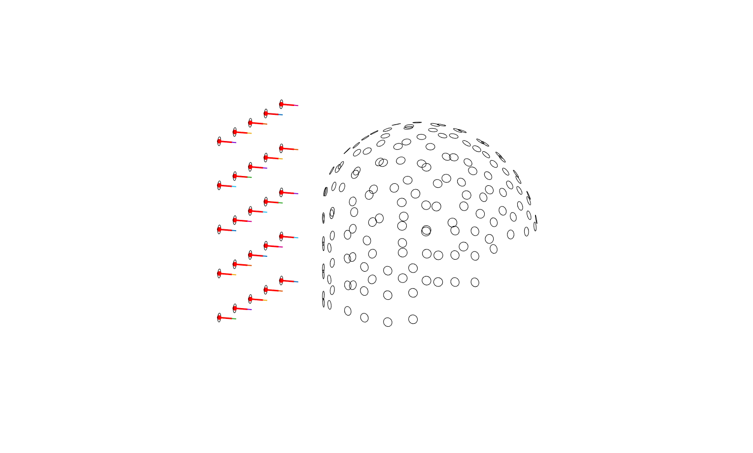
Cerca “Squalo”
Cerca has a PCB board with a 5x5 arrangement of magnetic dipole coils that I have seen in the MEG lab in Amsterdam. I don’t know the exact dimensions, so this is just an approximation.
% the following constructs a 20x20 cm grid placed posterior of the participant
% you can change this according to where you want the grid to be located
xgrid = linspace(-0.1, 0.1, 5);
ygrid = -0.2;
zgrid = linspace(-0.1, 0.1, 5);
[X, Y, Z] = ndgrid(xgrid, ygrid, zgrid);

phantom = [];
phantom.coilpos = [X(:) Y(:) Z(:)];
phantom.coilori = zeros(size(phantom.coilpos));
phantom.coilori(:,2) = 1;
phantom.label = arrayfun(@num2str, 1:size(phantom.coilpos,1), 'UniformOutput', false)';
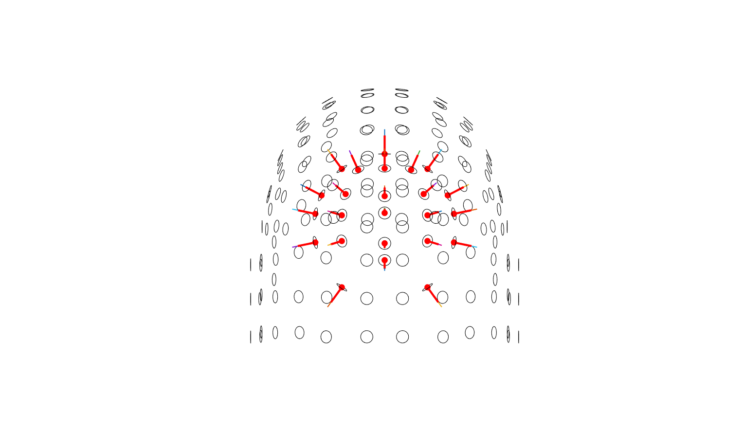
Spherical HPI array
At the DCCN we constructed an array with 24 HPI coils on a 120 mm diameter sphere that we use in combination with a 24-channel phantom current driver. More details will be posted soon on the open hardware page.
phantomcoil.unit = 'mm';
phantomcoil.coilpos = [
          0         0   60.0000
     0.0000   36.4237   47.6793
    34.6410   11.2555   47.6793
    21.4093  -29.4674   47.6793
   -21.4093  -29.4674   47.6793
   -34.6410   11.2555   47.6793
    31.5439   43.4164   26.8328
    51.0390  -16.5836   26.8328
     0.0000  -53.6656   26.8328
   -51.0390  -16.5836   26.8328
   -31.5439   43.4164   26.8328
     0.0000   58.9348   11.2555
    56.0503   18.2119   11.2555
    34.6410  -47.6793   11.2555
   -34.6410  -47.6793   11.2555
   -56.0503   18.2119   11.2555
    34.6410   47.6793  -11.2555
    56.0503  -18.2119  -11.2555
     0.0000  -58.9348  -11.2555
   -56.0503  -18.2119  -11.2555
   -34.6410   47.6793  -11.2555
     0.0000   53.6656  -26.8328
    34.6410  -11.2555  -47.6793
   -34.6410  -11.2555  -47.6793
];
phantomcoil.coilori = [
          0         0    1.0000
     0.0000    0.6071    0.7947
     0.5774    0.1876    0.7947
     0.3568   -0.4911    0.7947
    -0.3568   -0.4911    0.7947
    -0.5774    0.1876    0.7947
     0.5257    0.7236    0.4472
     0.8507   -0.2764    0.4472
    -0.0000   -0.8944    0.4472
    -0.8507   -0.2764    0.4472
    -0.5257    0.7236    0.4472
     0.0000    0.9822    0.1876
     0.9342    0.3035    0.1876
     0.5774   -0.7947    0.1876
    -0.5774   -0.7947    0.1876
    -0.9342    0.3035    0.1876
     0.5774    0.7947   -0.1876
     0.9342   -0.3035   -0.1876
    -0.0000   -0.9822   -0.1876
    -0.9342   -0.3035   -0.1876
    -0.5774    0.7947   -0.1876
     0.0000    0.8944   -0.4472
     0.5774   -0.1876   -0.7947
    -0.5774   -0.1876   -0.7947
];
phantomcoil.label = { '1', '2', '3', '4', '5', '6', '7', '8', '9', '10', '11', '12', '13', '14', '15', '16', '17', '18', '19', '20', '21', '22', '23', '24' };
Adachi sphere
Adashi and colleagues describe a spherical phantom in their 2023 paper “A Spherical Coil Array for the Calibration of Whole-Head Magnetoencephalograph Systems” that consists of large coils wrapped around a sphere. At the DCCN we constructed one based on a 3D-printed sphere with 120 mm diameter. This phantom can be described with the following geometry, where the center of each coil is teh same as the center of the sphere.
phantom = [];
phantom.unit = 'm';
phantom.coilpos = zeros(16,3);
phantom.coilori = [
          0         0    1.0000
     0.8944         0    0.4472
     0.2764   -0.8507    0.4472
    -0.7236   -0.5257    0.4472
    -0.7236    0.5257    0.4472
     0.2764    0.8507    0.4472
     0.4911   -0.3568    0.7947
    -0.1876   -0.5774    0.7947
    -0.6071         0    0.7947
    -0.1876    0.5774    0.7947
     0.4911    0.3568    0.7947
     0.7947   -0.5774    0.1876
     0.3035   -0.9342   -0.1876
    -0.3035   -0.9342    0.1876
    -0.7947   -0.5774   -0.1876
    -0.9822         0    0.1876
    ];
phantom.label = { '1', '2', '3', '4', '5', '6', '7', '8', '9', '10', '11', '12', '13', '14', '15', '16'}';
Each of the 16 coils has a diameter of 120 mm. To plot these correctly with ft_plot_sens, you have to specify a a coilsize of 120 mm.
All other phantoms considered here have very small HPI-like coils that we model as a magnetic dipole. For most EEG and MEG volume conduction models the ft_compute_leadfield will assume that the source is an equivalent current dipole (ECD). When we specify the volume conductor type as as “infinite” and pass a MEG sensor array rather than an EEG electrode array, it will compute the leadfield for a magnetic dipole.
To compute the leadfield matrix (i.e. the topography for a coil in the x, y, and z-direction) for a coil of a specific size, we have to specify the size in the headmodel. So to compute the topography for coils wrapped around the 120 mm diameter sphere, you have to specify the following headmodel:
headmodel = [];
headmodel.type = 'circularcoil';
headmodel.diameter = 0.12;
headmodel.unit = 'm';
Visualize the phantom coils together with the OPM sensors
The following code can be used with all phantom structures that we created above. The coil size that is plotted is not geometrically correct, but set to 10 mm to make it easier to see the coil and orientation. For the Adachi sphere the coil size should be specified as 120 mm.
figure
ft_plot_sens(fieldlinebeta2, 'axes', false, 'fiducial', false)
ft_plot_sens(phantom, 'coil', true, 'orientation', false, 'coilsize', 0.01)
% ft_plot_sens(phantom, 'label', 'label')
ft_plot_dipole(phantom.coilpos, phantom.coilori', 'unit', 'm')
Compute and plot the phantom coil topographies
The following code (with some minor changes) can be used with all phantom structures that we created above.
% compute actual magnetic field values in SI units
diameter = 0.006;
turns    = 3;
area     = pi*(diameter/2)^2;
current  = 5 / 200000; % 5V peak-to-peak over a 200 kOhm resistor
mom      = turns * area * current;

nchans = length(fieldlinebeta2.label);
ncoils = length(phantom.label);

dat = zeros(nchans, ncoils);
for i=1:ncoils
    dat(:,i) = ft_compute_leadfield(phantom.coilpos(i,:), fieldlinebeta2, headmodel) * mom * phantom.coilori(i,:)';
end

m = max(abs(dat(:)));
fprintf('max field is %f pT\n', m * 1e12)

figure
clear ax
n = ceil(sqrt(length(phantom.label)));

for i=1:ncoils
    ax(i) = subplot(n,n,i);
    ft_plot_topo3d(fieldlinebeta2.coilpos, dat(:,i), 'refine', 1);
    ft_colormap('-RdBu')
    ft_plot_sens(fieldlinebeta2, 'fiducial', false)
    ft_plot_sens(phantom, 'chanindx', i, 'coil', true, 'orientation', true, 'coilsize', diameter);
    ft_plot_dipole(phantom.coilpos(i,:), phantom.coilori(i,:)', 'unit', 'm')
    clim([-m m])
end

linkprop(ax, {'CameraPosition', 'CameraUpVector'});
rotate3d on
This is the image you get for the HPI coils on the anatomical landmarks.
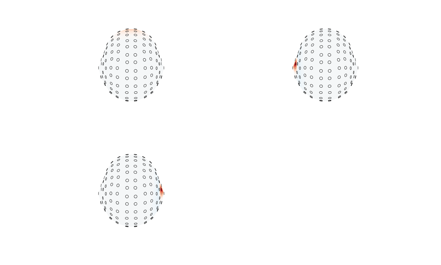
You should rotate the helmet topographies to get a correct 3D representation of the OPMs, the phantom coils, and their topographies. For the configurations with more phantoms coils this is difficult to capture in a screen shot, so please compute and plot them yourself.