Symmetric dipole pairs for beamforming
When you expect symmetric activity in an ERP analysis, it makes sense to use a symmetric dipole pair in ft_dipolefitting by specifying the cfg.symmetry option. For the scanning methods that are implemented in ft_sourceanalysis, and notably for the beamformer methods, you can also make use of symmetric dipole pairs.
This is especially beneficial when the source activity in left and right hemisphere is expected to be highly correlated, as the beamformer expects sources to be (reasonably) uncorrelated. By extending the sourcemodel, the source activity that you are simultaneously estimating while scanning includes both left and right hemisphere activity and the correlation inside that sourcemodel is not a problem.
Simulation of correlated and un-correlated symmetric dipole pairs
To investigate the effects of applying a symmetry constraint to the beamformer analysis, we will simulate two scenarios of symmetric dipoles; correlated and un-correlated. We will then attempt to estimate them with and without symmetry constraints. There coherent simulation script is available here.
First, the symmetric dipoles and a spherical volume conductor model are defined:
% Define two dipole positions and two directions of moment
dippos = [-4 -4 4; 4 -4 4];
dipmom = [1 0 .5; -1 0 .5]';

% Create an array with some magnetometers at 12cm distance from the origin
[X, Y, Z] = sphere(10);
pos = unique([X(:) Y(:) Z(:)], 'rows');
pos = pos(pos(:,3)>=0,:);
grad = [];
grad.coilpos = 12*pos;
grad.coilori = pos; % in the outward direction

for i=1:length(pos)
grad.label{i} = sprintf('chan%03d', i);
end

% Create a spherical volume conductor with 10cm radius
vol.r = 10;
vol.o = [0 0 0];
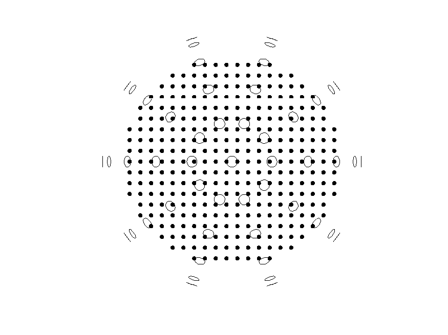
Then, a ‘normal’ non-symmetric source model is defined, and the grid is plotted:
% Define a non-symmetric 'normal' source model
cfg = [];
cfg.headmodel = vol; % use the spherical volume conductor as head model
cfg.grad = grad;
% Source models are defined with x-axis normal to the midline.
cfg.xgrid = -9.5:9.5; % ensure that the midline is not included
cfg.ygrid = -10:10;
cfg.zgrid = 0:10;
sourcemodel_normal = ft_prepare_leadfield(cfg);

% Plot the grid of the source model
figure
ft_plot_mesh(sourcemodel_normal.pos(sourcemodel_normal.inside,:))
ft_plot_sens(grad)
Un-correlated symmetric sources with non-symmetric source model
Two conditions are defined with uncorrelated (i.e. phase shifted) symmetric 40 Hz signals of varying amplitude emulating a left and right lateral attention modulation. Note that the left dipole signal is defined by a sin while the right is defined by a cos.
% Dipole simulation
cfg = [];
cfg.headmodel = vol;
cfg.grad = grad;
cfg.fsample = 1000;
cfg.relnoise = 2;
cfg.sourcemodel.pos = dippos(:,:);
cfg.sourcemodel.mom = dipmom(:,:);
% create some left-right amplitude imbalance, emulating lateral attention modulation
cfg.sourcemodel.signal = repmat({[1.1*sin(40*2*pi*(0:999)/1000); 0.9*cos(40*2*pi*(0:999)/1000)]}, 1, 10);
dataLR_attL = ft_dipolesimulation(cfg);
cfg.sourcemodel.signal = repmat({[0.9*sin(40*2*pi*(0:999)/1000); 1.1*cos(40*2*pi*(0:999)/1000)]}, 1, 10);
dataLR_attR = ft_dipolesimulation(cfg);
Compute the data covariance matrix, which will capture the activity of each simulated dipole and is needed for the beamformer source estimation:
cfg = [];
cfg.covariance = 'yes';
timelockLR_attL  = ft_timelockanalysis(cfg, dataLR_attL);
timelockLR_attR  = ft_timelockanalysis(cfg, dataLR_attR);
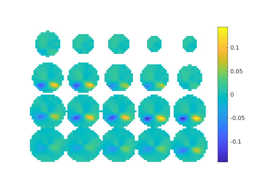
Apply the beamformer based on the non-symmetric ‘normal’ source model, calculate the lateral contrast, and plot the result:
cfg = [];
cfg.headmodel = vol;
cfg.grad = grad;
cfg.sourcemodel = sourcemodel_normal;
cfg.method = 'lcmv';
singleLR_attL = ft_sourceanalysis(cfg, timelockLR_attL);
singleLR_attR = ft_sourceanalysis(cfg, timelockLR_attR);

cfg           = [];
cfg.operation = '(x2-x1)/(x1+x2)'; % right minus left
cfg.parameter = 'pow';
contrastLR_attL_attR = ft_math(cfg, singleLR_attL, singleLR_attR);

cfg = [];
cfg.method = 'slice';
cfg.funparameter = 'pow';
figure; ft_sourceplot(cfg, contrastLR_attL_attR);
Correlated symmetric sources with non-symmetric source model
Now, let’s make the oscillations of the two symmetric dipoles correlated by changing the right dipole signals from cosines to sines:
% Dipole simulation
cfg = [];
cfg.headmodel = vol;
cfg.grad = grad;
cfg.fsample = 1000;
cfg.relnoise = 2;
cfg.sourcemodel.pos = dippos(:,:);
cfg.sourcemodel.mom = dipmom(:,:);
% create some left-right amplitude imbalance, emulating lateral attention modulation.
% OBS: Notice the right dipole signal is now also defined by a sine
cfg.sourcemodel.signal = repmat({[1.1*sin(40*2*pi*(0:999)/1000); 0.9*sin(40*2*pi*(0:999)/1000)]}, 1, 10);
dataLR_attL = ft_dipolesimulation(cfg);
cfg.sourcemodel.signal = repmat({[0.9*sin(40*2*pi*(0:999)/1000); 1.1*sin(40*2*pi*(0:999)/1000)]}, 1, 10);
dataLR_attR = ft_dipolesimulation(cfg);
Compute the covariance and apply the beamformer still with the non-symmetric source model:
cfg = [];
cfg.covariance = 'yes';
timelockLR_attL  = ft_timelockanalysis(cfg, dataLR_attL);
timelockLR_attR  = ft_timelockanalysis(cfg, dataLR_attR);

cfg = [];
cfg.headmodel = vol;
cfg.grad = grad;
cfg.sourcemodel = sourcemodel_normal;
cfg.method = 'lcmv';
singleLR_attL = ft_sourceanalysis(cfg, timelockLR_attL);
singleLR_attR = ft_sourceanalysis(cfg, timelockLR_attR);

cfg           = [];
cfg.operation = '(x2-x1)/(x1+x2)'; % right minus left
cfg.parameter = 'pow';
contrastLR_attL_attR = ft_math(cfg, singleLR_attL, singleLR_attR);

cfg = [];
cfg.method = 'slice';
cfg.funparameter = 'pow';
figure; ft_sourceplot(cfg, contrastLR_attL_attR);
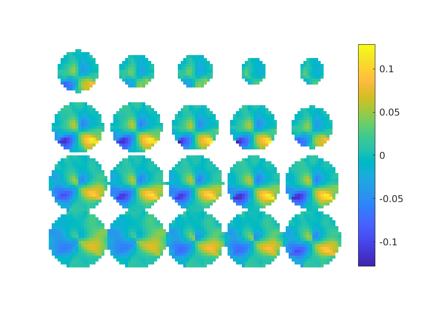
Due to the correlation between the spatially separated source signals, the LCMV estimator produces a sub-optimal spatial filter that is less sensitive to both sources.
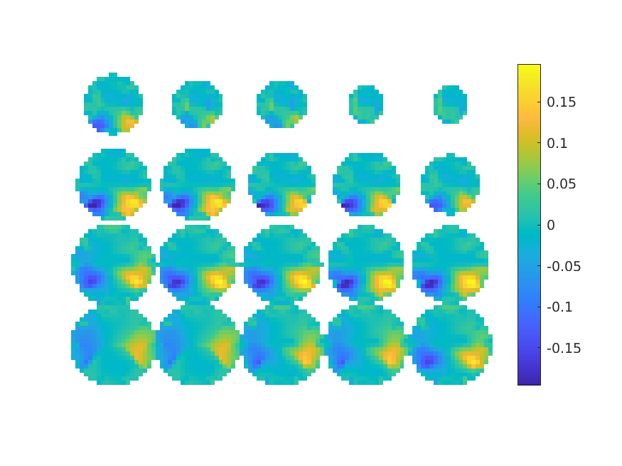
Correlated symmetric sources with symmetric source model
To deal with the correlation between the symmetric dipoles, the source model is re-defined with a symmetry constraint across the midline (in this case the x-axis):
% Source model with symmetry constraint over the midline.
cfg = [];
cfg.headmodel = vol;
cfg.grad = grad;
cfg.xgrid = -9.5:0; % Only define one hemisphere
cfg.ygrid = -10:10;
cfg.zgrid = 0:10;
cfg.symmetry = 'x'; % Axis of symmetry - OBS: This is dependent on scanner coordinate system
sourcemodel_double = ft_prepare_leadfield(cfg);
In the symmetric sourcemodel, the .pos field is a N/2x6 matrix (where N is the number of vertices in the grid), rather than the usual Nx3, where the xyz-coordinates of the vertices are given in pairs of triplets.
>> head(sourcemodel_double.pos)
    -9.5000   -9.0000         0    9.5000   -9.0000         0
    -8.5000   -9.0000         0    8.5000   -9.0000         0
    -7.5000   -9.0000         0    7.5000   -9.0000         0
    -6.5000   -9.0000         0    6.5000   -9.0000         0
    -5.5000   -9.0000         0    5.5000   -9.0000         0
    -4.5000   -9.0000         0    4.5000   -9.0000         0
    -3.5000   -9.0000         0    3.5000   -9.0000         0
    -2.5000   -9.0000         0    2.5000   -9.0000         0
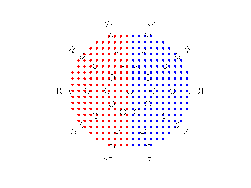
Plot the symmetrically defined grid, colour coding each hemisphere:
figure
ft_plot_mesh(sourcemodel_double.pos(sourcemodel_double.inside,1:3), 'vertexcolor', 'r')
ft_plot_mesh(sourcemodel_double.pos(sourcemodel_double.inside,4:6), 'vertexcolor', 'b')
ft_plot_sens(grad)
Re-do the beamformer estimation with the symmetric source model
cfg = [];
cfg.headmodel = vol;
cfg.grad = grad;
cfg.sourcemodel = sourcemodel_double;
cfg.method = 'lcmv';
singleLR_attL = ft_sourceanalysis(cfg, timelockLR_attL);
singleLR_attR = ft_sourceanalysis(cfg, timelockLR_attR);
Now, the source estimates need to be reshaped from the symmetrically defined source model to the normal source model dimensions:
% construct the single-dipole model from the (symmetric) double-dipole model
n = size(sourcemodel_double.pos,1);
lh2full = nan(n,1);
rh2full = nan(n,1);

% determine the mapping between the left and right hemisphere to the full model
for i=1:n
    pos_lh = sourcemodel_double.pos(i,1:3); % Left hemisphere positions
    pos_rh = sourcemodel_double.pos(i,4:6); % Right hemisphere positions
    lh2full(i) = find(sourcemodel_normal.pos(:,1)==pos_lh(1) & sourcemodel_normal.pos(:,2)==pos_lh(2) & sourcemodel_normal.pos(:,3)==pos_lh(3));
    rh2full(i) = find(sourcemodel_normal.pos(:,1)==pos_rh(1) & sourcemodel_normal.pos(:,2)==pos_rh(2) & sourcemodel_normal.pos(:,3)==pos_rh(3));
end

% this mainly serves as a sanity check
sourcemodel_single = [];
sourcemodel_single.pos(lh2full, 1) = sourcemodel_double.pos(:,1);
sourcemodel_single.pos(lh2full, 2) = sourcemodel_double.pos(:,2);
sourcemodel_single.pos(lh2full, 3) = sourcemodel_double.pos(:,3);
sourcemodel_single.pos(rh2full, 1) = sourcemodel_double.pos(:,4);
sourcemodel_single.pos(rh2full, 2) = sourcemodel_double.pos(:,5);
sourcemodel_single.pos(rh2full, 3) = sourcemodel_double.pos(:,6);

% these should now be equal
assert(isequal(sourcemodel_single.pos, sourcemodel_normal.pos));

sourcemodel_single.dim = sourcemodel_normal.dim;
sourcemodel_single.unit = sourcemodel_normal.unit;
sourcemodel_single.inside = sourcemodel_normal.inside;

% convert the (symmetric) double-dipole estimates into a single-dipole representation
singleLR_attL = sourcemodel_single;
singleLR_attL.pow = nan(prod(sourcemodel_normal.dim),1);
singleLR_attR = sourcemodel_single;
singleLR_attR.pow = nan(prod(sourcemodel_normal.dim),1);
Extract the covariance from each hemisphere and calculate the power using the first singular value:
for i=find(doubleLR_attL.inside(:)')
    covL = doubleLR_attL.avg.cov{i}(1:3,1:3); % Left hemisphere covariance
    covR = doubleLR_attL.avg.cov{i}(4:6,4:6); % Right hemisphere covariance
    powL = svd(covL); powL = powL(1); % Estimate power by 1st singular value
    powR = svd(covR); powR = powR(1);
    singleLR_attL.pow(lh2full(i)) = powL;
    singleLR_attL.pow(rh2full(i)) = powR;

    covL = doubleLR_attR.avg.cov{i}(1:3,1:3);
    covR = doubleLR_attR.avg.cov{i}(4:6,4:6);
    powL = svd(covL); powL = powL(1);
    powR = svd(covR); powR = powR(1);
    singleLR_attR.pow(lh2full(i)) = powL;
    singleLR_attR.pow(rh2full(i)) = powR;
end
Compute the contrast between the conditions as before and plot the results
cfg           = [];
cfg.operation = '(x2-x1)/(x1+x2)'; % right minus left
cfg.parameter = 'pow';
contrastLR_attL_attR = ft_math(cfg, singleLR_attL, singleLR_attR);

cfg = [];
cfg.method = 'slice';
cfg.funparameter = 'pow';
figure; ft_sourceplot(cfg, contrastLR_attL_attR);

Un-correlated symmetric sources with symmetric source model
Finally, we show the effect of using a symmetric source model to estimate two un-correlated symmetric sources:
% Dipole simulation
cfg = [];
cfg.headmodel = vol;
cfg.grad = grad;
cfg.fsample = 1000;
cfg.relnoise = 2;
cfg.sourcemodel.pos = dippos(:,:);
cfg.sourcemodel.mom = dipmom(:,:);
% create some left-right amplitude imbalance, emulating lateral attention modulation.
% OBS: Notice the right dipole signal is now also defined by a sine
cfg.sourcemodel.signal = repmat({[1.1*sin(40*2*pi*(0:999)/1000); 0.9*cos(40*2*pi*(0:999)/1000)]}, 1, 10);
dataLR_attL = ft_dipolesimulation(cfg);
cfg.sourcemodel.signal = repmat({[0.9*sin(40*2*pi*(0:999)/1000); 1.1*cos(40*2*pi*(0:999)/1000)]}, 1, 10);
dataLR_attR = ft_dipolesimulation(cfg);

% Compute covariance
cfg = [];
cfg.covariance = 'yes';
timelockLR_attL  = ft_timelockanalysis(cfg, dataLR_attL);
timelockLR_attR  = ft_timelockanalysis(cfg, dataLR_attR);

% Do symmetric source estimation
cfg = [];
cfg.headmodel = vol;
cfg.grad = grad;
cfg.sourcemodel = sourcemodel_double;
cfg.method = 'lcmv';
singleLR_attL = ft_sourceanalysis(cfg, timelockLR_attL);
singleLR_attR = ft_sourceanalysis(cfg, timelockLR_attR);

% convert the (symmetric) double-dipole estimates into a single-dipole representation
singleLR_attL = sourcemodel_single;
singleLR_attL.pow = nan(prod(sourcemodel_normal.dim),1);
singleLR_attR = sourcemodel_single;
singleLR_attR.pow = nan(prod(sourcemodel_normal.dim),1);

% Extract the covariance from each hemisphere and calculate the power using the first singular value:
for i=find(doubleLR_attL.inside(:)')
    covL = doubleLR_attL.avg.cov{i}(1:3,1:3); % Left hemisphere covariance
    covR = doubleLR_attL.avg.cov{i}(4:6,4:6); % Right hemisphere covariance
    powL = svd(covL); powL = powL(1); % Estimate power by 1st singular value
    powR = svd(covR); powR = powR(1);
    singleLR_attL.pow(lh2full(i)) = powL;
    singleLR_attL.pow(rh2full(i)) = powR;

    covL = doubleLR_attR.avg.cov{i}(1:3,1:3);
    covR = doubleLR_attR.avg.cov{i}(4:6,4:6);
    powL = svd(covL); powL = powL(1);
    powR = svd(covR); powR = powR(1);
    singleLR_attR.pow(lh2full(i)) = powL;
    singleLR_attR.pow(rh2full(i)) = powR;
end

% Compute contrast
cfg           = [];
cfg.operation = '(x2-x1)/(x1+x2)'; % right minus left
cfg.parameter = 'pow';
contrastLR_attL_attR = ft_math(cfg, singleLR_attL, singleLR_attR);

% Plot source contrasts
cfg = [];
cfg.method = 'slice';
cfg.funparameter = 'pow';
figure; ft_sourceplot(cfg, contrastLR_attL_attR);
Example auditory steady state response
The use of symmetric dipoles is explained for Steady State Auditory Potentials (SSAEPs) in the paper by Tzvetan Popov, Robert Oostenveld, Jan M. Schoffelen (2018) FieldTrip Made Easy: An Analysis Protocol for Group Analysis of the Auditory Steady State Brain Response in Time, Frequency, and Space. Supporting material, including all data and scripts can be found on the Radboud Data Repository.
The following excerpts from ASSR_dics.m (download) make up the analysis pipeline of the SSAEPs from Popov et. al. 2018 using symmetric dipoles and Dynamic imaging of coherent sources (DICS). The SSAEP is a very high SNR signal, leading to (near) simultaneous (i.e. zero-lag correlated) activation in bilateral auditory areas. Therefore, the traditional beamformer will fail to yield good results. Note that the excerpts here present the method on a single subject, while ASSR_dics.m provide the analysis across subjects as well.
Configure data and FieldTrip paths, and specify some study metadata:
% initialize fieldtrip
path_ft   = '/path/to/fieldtrip';
path_data = '/path/to/data/ASSR';

% this adds fieldtrip to the matlab path + the relevant subdirectories
addpath(path_ft);
ft_defaults;

% we choose a single subject for demonstration purposes
subject = '45048'
Load in the precomputed geometric data that is needed for source reconstruction: the forward model (leadfields), as well as the volume conductor model of the head, and the electrodes. Strictly speaking, once the forward model is available, the other objects are not needed anymore, but FieldTrip expects them to be present in the cfg.
load(fullfile(path_data,'templates','headmodel.mat'));
load(fullfile(path_data,'templates','leadfield.mat'));
load(fullfile(path_data,'templates','elec_aligned.mat'));
In this example here, we have already computed leadfields, so we will create for each original dipole location a leadfield consisting of a concatenation of this dipole’s leadfield with its counterpart in the opposite hemisphere. Note that the x-coordinate here is the left/right direction.
lf1 = reshape(leadfield.leadfield, leadfield.dim);
lf2 = flip(lf1,1);
for k = 1:numel(lf1)
    if ~isempty(lf1{k})&&~isempty(lf2{k})
        leadfield.leadfield{k} = [lf1{k} lf2{k}];
    else
        leadfield.leadfield{k} = [];
        leadfield.inside(k)    = false;
    end
end
clear lf1 lf2
Load the data and divide it into pre and post stimulus segments. We also concatenate the two for the purpose of estimating a common spatial filter.
datafile = fullfile(path_data, 'data', subject, 'data.mat');
load(datafile)

% remove bad channels
cfg         = [];
cfg.channel = {'all' '-E30' '-E3' '-E4' '-E11' '-E12' '-Cz' '-E192'};
data        = ft_selectdata(cfg, data);

% this chunk of code creates a 'dummy' reference channel to be used for
% the coherence analysis
trial = cell(size(data.trial));
for k = 1:numel(trial)
    trial{k} = sin(2.*pi.*40.*data.time{k});
end
refdata.trial = trial;
refdata.time  = data.time;
refdata.label = {'refchan'};
data          = ft_appenddata([], data, refdata);
data.fsample  = 1000;

% re-segment the data into pre and post stimulus onset intervals
cfg        = [];
cfg.toilim = [-1 0-1./data.fsample];
datapre    = ft_redefinetrial(cfg, data);

cfg.toilim = [1 2-1./data.fsample];
datapost   = ft_redefinetrial(cfg, data);

% append data to facilitate the computation of a 'common' spatial filter
dataall = ft_appenddata([], datapre, datapost);
The cross-spectral density matrices are calculated for each of the two conditions and the concatenated data. Here, we focus on the 40 Hz component:
cfg        = [];
cfg.method = 'mtmfft';
cfg.output = 'fourier';
cfg.taper  = 'hanning';
cfg.foilim = [40 40];
freqpre    = ft_freqanalysis(cfg, datapre);
freqpost   = ft_freqanalysis(cfg, datapost);
freqall    = ft_freqanalysis(cfg, dataall);

% the data consists of fewer channels than the precomputed
% leadfields, the following chunk of code takes care of this
[a,b] = match_str(data.label, leadfield.label);
for k = 1:numel(leadfield.leadfield)
    if ~isempty(leadfield.leadfield{k})
        tmp = leadfield.leadfield{k};
        tmp = tmp(b,:);
        tmp = tmp-repmat(mean(tmp,1),[size(tmp,1) 1]); % average re-ref
        leadfield.leadfield{k} = tmp;
    end
end
leadfield.label = leadfield.label(b);
Perform source reconstruction using the DICS method . Note that cfg.dics.keepfilter = 'yes' allows us to pass the estimated spatial filter to the subsequent source analysis of individual conditions.
cfg                   = [];
cfg.method            = 'dics';
cfg.frequency         = 40;
cfg.channel           = data.label;
cfg.elec              = elec_aligned;
cfg.grid              = leadfield;
cfg.headmodel         = headmodel;
cfg.dics.keepfilter   = 'yes';
cfg.dics.fixedori     = 'no';
cfg.dics.projectnoise = 'yes';
cfg.dics.lambda       = '5%';
cfg.dics.realfilter   = 'yes';
cfg.dics.keepcsd      = 'yes';
cfg.refchan           = {'refchan'};
sourceall             = ft_sourceanalysis(cfg, freqall);

% apply common filters to pre and post stimulus data
cfg.grid.filter = sourceall.avg.filter;
Now we need to extract the dipole pairs’ full csd matrix with respect to the reference channel, which is not possible in the traditional DICS implementation, but can be achieved with PCC
cfg.method   = 'pcc';
cfg          = rmfield(cfg, 'dics');
sourcepre    = ft_sourceanalysis(cfg, freqpre);
sourcepst    = ft_sourceanalysis(cfg, freqpost);
Now we need to adjust the ‘csdlabel’, in order to compute the single dipole-of-interest coherence with the reference. source.avg.csd contains for each dipole pair the cross-spectral density as a 7x7 matrix, two triplets of rows/columns for each of the dipoles in the pair, and one for the reference signal. ft_sourcedescriptives will return the coherence between the ‘scandip’ and the ‘refchan’, so we need to relabel the second dipole’s label
for k = 1:size(sourcepre.pos,1)
    if ~isempty(sourcepre.avg.csdlabel{k})
        sourcepre.avg.csdlabel{k}(4:6) = {'supdip'};
        sourcepst.avg.csdlabel{k}(4:6) = {'supdip'};
    end
end
sourcepre = ft_sourcedescriptives([], sourcepre);
sourcepst = ft_sourcedescriptives([], sourcepst);
Contrast post stimulus onset activity with respect to baseline
cfg           = [];
cfg.operation = 'x2-x1';
cfg.parameter = 'avg.coh';
source_dics   = ft_math(cfg,sourcepre,sourcepst);