Using threshold-free cluster enhancement for cluster statistics
This example explains how the threshold-free cluster enhancement (TFCE) method works for cluster statistics.
Why is it useful?
When using clusting to correct for multiple comparisons, we need to define the cluster-forming threshold using the cfg.clusterthreshold and the cfg.clusteralpha options in ft_statistics_montecarlo. Different clusteralpha thresholds lead to clusters with a different spatial ot temporal extent, and thereby potentially to a different sensitivity of the subsequent permutation test. The threshold-free cluster enhancement method (TFCE) was introduced by Smith and Nichols (2009) to overcome this arbitrary threshold.
How does it work?
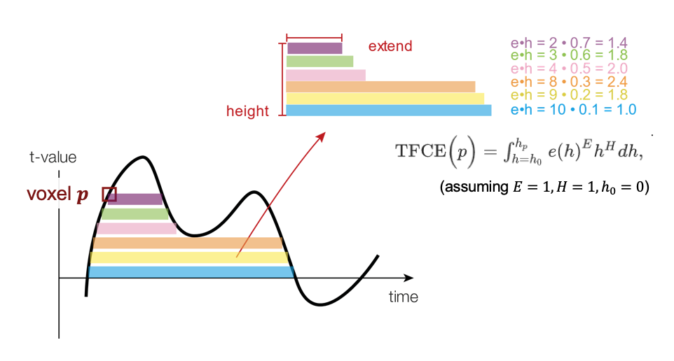
Each voxel’s TFCE score is given by the sum of the scores of all “supporting sections” underneath it; as the height 𝒉 is incrementally raised from zero up to the height (signal intensity) 𝒉p of a given point 𝒑, the image is thresholded at 𝒉, and the single contiguous cluster containing p is used to define the score for that height 𝒉. This score is simply the height 𝒉 (raised to some power 𝑯, which is by default set to 2 in FieldTrip and can be adjusted via cfg.tfce_H) multiplied by the cluster extent 𝒆 (raised to some power 𝑬, which is by default set to 0.5 in FieldTrip and can be adjusted via cfg.tfce_E). For more detailed information, see Smith and Nichols (2009).
TFCE schematic, adapted from Benedikt V. Ehinger (used under CC-BY)
Example code
The following MATLAB code gives an example of the TFCE method. Moreover, we will compare the statistical output of the TFCE method with the conventional threshold based on cfg.clusteralpha.
The data used in this example is available from our download server.
load ERF_orig

Nsubj       = 10;
design      = zeros(2, Nsubj*2);
design(1,:) = [1:Nsubj 1:Nsubj];                % this is the uvar (unit-of-observation variable)
design(2,:) = [ones(1,Nsubj) ones(1,Nsubj)*2];  % this is the ivar (independent variable)

% channel neighbours are not really needed for the subsequent example, since we restrict the test to a single channel
% nevertheless, we will determine the channel neighbours here anyway
cfg          = [];
cfg.method   = 'template';
cfg.template = 'CTF151_neighb.mat';
nb           = ft_prepare_neighbours( cfg, allsubjFIC{1} );

%% Conventional cluster-based permutation test
cfg                  = [];
cfg.design           = design;
cfg.uvar             = 1;
cfg.ivar             = 2;
cfg.channel          = {'MLT12'};
cfg.latency          = [0 1];
cfg.method           = 'montecarlo';
cfg.statistic        = 'depsamplesT';
cfg.numrandomization = 'all';   % there are 10 subjects, so 2^10=1024 possible raondomizations
cfg.tail             = 0;
cfg.alpha            = 0.025;   % since we are testing two tails
cfg.neighbours       = nb;      % this will not be used, since we selected only a single channel
cfg.correctm         = 'cluster';
cfg.clusterstatistic = 'maxsum';
cfg.clusterthreshold = 'nonparametric_individual';
cfg.clustertail      = 0;
cfg.clusteralpha     = 0.01;
stat01 = ft_timelockstatistics(cfg, allsubjFIC{:}, allsubjFC{:});

cfg.clusteralpha     = 0.05;
stat05 = ft_timelockstatistics(cfg, allsubjFIC{:}, allsubjFC{:});

%% Cluster-based permutation test with TFCE method
cfg                  = [];
cfg.design           = design;
cfg.uvar             = 1;
cfg.ivar             = 2;
cfg.channel          = {'MLT12'};
cfg.latency          = [0 1];
cfg.method           = 'montecarlo';
cfg.statistic        = 'depsamplesT';
cfg.numrandomization = 'all';   % there are 10 subjects, so 2^10=1024 possible raondomizations
cfg.tail             = 0;
cfg.alpha            = 0.025;   % since we are testing two tails
cfg.neighbours       = nb;      % this will not be used, since we selected only a single channel
cfg.correctm         = 'tfce';
cfg.tfce_H           = 2;       % default setting
cfg.tfce_E           = 0.5;     % default setting
statA = ft_timelockstatistics(cfg, allsubjFIC{:}, allsubjFC{:});

cfg.tfce_H           = 2;
cfg.tfce_E           = 0.25;
statB = ft_timelockstatistics(cfg, allsubjFIC{:}, allsubjFC{:});
Note that the TFCE method takes longer to compute than the conventional method. We can visualize and compare the slightly different statistical outputs given by these methods.
%% Visualize the results
figure(1), clf, hold on,
set(gcf, 'units','centimeters','position',[0 0 18 10] );
subplot(2,2,1), hold on, grid on,
title( 'TFCE: H=2, E=0.5' );
plot( statA.time, statA.stat_tfce, 'r');
plot( statA.time(statA.mask), 400*ones(sum(statA.mask),1), 'r', 'linewidth',2 );
ylabel( 'TFCE' );
ylim( [-20, 420] );
xticks( 0:0.2:1 );
set(gca, 'TickDir','out' );

subplot(2,2,3), hold on, grid on,
title( 'TFCE: H=2, E=0.25' );
plot( statB.time, statB.stat_tfce, 'r');
plot( statB.time(statB.mask), 400*ones(sum(statB.mask),1), 'r', 'linewidth',2 );
ylabel( 'TFCE' );
ylim( [-20, 420] );
xticks( 0:0.2:1 );
set(gca, 'TickDir','out' );

subplot(2,2,2), hold on, grid on,
title( 'clusteralpha = .01' );
plot( stat01.time, stat01.stat, 'k');
plot( stat01.time(stat01.mask), 7.5*ones(sum(stat01.mask),1), 'k', 'linewidth',2 );
ylabel( 't-value' );
ylim( [-3, 8] );
xticks( 0:0.2:1 );
set(gca, 'TickDir','out' );

subplot(2,2,4), hold on, grid on,
title( 'clusteralpha = .05' );
plot( stat05.time, stat05.stat, 'k');
plot( stat05.time(stat05.mask), 7.5*ones(sum(stat05.mask),1), 'k', 'linewidth',2 );
ylabel( 't-value' );
ylim( [-3, 8] );
xticks( 0:0.2:1 );
set(gca, 'TickDir','out' );
Output of the example code
When you inspect stat01, stat05, statA and statB, you will see that in this case the null-hypothesis of exchangeability of the data over the two conditions is rejected in all four.
Here is the expected output of the example code.

