Getting started with SimNIBS

Background

SimNIBS is a free and open source software package for Simulation of Non-invasive Brain Stimulation. Besides allowing for calculations of the electric field induced by transcranial magnetic stimulation (TMS) and transcranial electric stimulation (TES), the methods implemented in SimNIBS can also be used for electroencephalography (EEG) forward modeling. We refer to Nielsen et al. (2023) for more information about using SimNIBS for EEG forward calculations.

Procedure

In this tutorial we will use SimNIBS to solve the forward problem in EEG for a specific subject. The end result is a matrix (often called the leadfield or gain matrix) which maps source activations to sensor readings. The procedure consists of four steps:

• Generate a physical model of the head. We rely on one (or two) subject-specific MR image(s) for this.
• Convert electrode locations to SimNIBS readable format.
• Calculate a TDCS (transcranial direct current stimulation) leadfield matrix. (This is known as the reciprocal approach.)
• Calculate the final EEG leadfield matrix.

Below, we provide more details on each of these steps and show the necessary commands to execute. We will use the same dataset as is used in the this FEM tutorial (which provides a little more background on the forward problem itself). We will be using FieldTrip and SimNIBS, hence you will need to call functions from within MATLAB as well as your shell of choice (command line calls). A prefix to each code block indicates where the code is to be executed. For the SimNIBS command line calls to be valid, you need to have SimNIBS installed and in your PATH.

Note that we have used SimNIBS 4.0.1 for this tutorial.

Preparation

We will need Subject01.mri which you can get here. For the remainder of this tutorial we will assume that this file is present in the current working directory (to which all paths mentioned here are relative). Let us start by converting the MR image to the RAS coordinate system (it is initially CTF) and save it in a standard NIfTI format that can be read by SimNIBS. (If your image is already in NIfTI format, this should not be necessary.)

% matlab
ft_defaults;

mri_in = 'Subject01.mri';
mri_out = 'Subject01.nii.gz';

mri = ft_read_mri(mri_in);
mri = ft_convert_coordsys(mri, 'ras'); % this relies on the SPM toolbox
ft_write_mri(mri_out, mri);

Generating the head model

In order to create a (realistic) head model, we will need a subject-specific MR image. If a single image is used, this will often be T1-weighted as this provides great contrast between cortical tissues. However, SimNIBS offers the possibility to supply an additional contrast to improve the anatomical accuracy of the resulting model. We usually recommend a T2-weighted scan as this provides a nice contrast between bone and cerebrospinal fluid (CSF). If possible, supplying both a T1- and a T2-weighted image is highly recommended. However, for this particular subject, we only have a T1-weighted scan. SimNIBS also needs a subject ID for its data. Here, we will simply use Subject01.

The segmentation and meshing tool in SimNIBS is called charm. Running this will create a folder called m2m_Subject01 in the directory from which the command is executed.

# shell
charm Subject01 Subject01.nii.gz --forceqform

This will run all necessary steps (segmentation, meshing, brain surface extraction) and should take approximately 1-2 hours to complete. It generates multiple files, however, of particular relevance to us is the tetrahedral head mesh (m2m_Subject01/Subject01.msh) and the central surfaces of the left and right cerebral cortices (located in m2m_Subject01/surfaces) which we will use to define the source space.

It is always advised to visually check the accuracy of the results before continuing. For this purpose, you may want to consult the html report (m2m_Subject01/charm_report.html) or use your preferred visualization tool and overlay final_tissues.nii.gz on T1.nii.gz. It is also possible to manually edit the segmentation before the meshing.

Figure. Segmentation (borders) overlaid on the T1-weighted image. This MR image has a rather low resolution (1.25 mm isotropic voxels), however, the skull (compact and spongy bone) is still captured reasonably well.

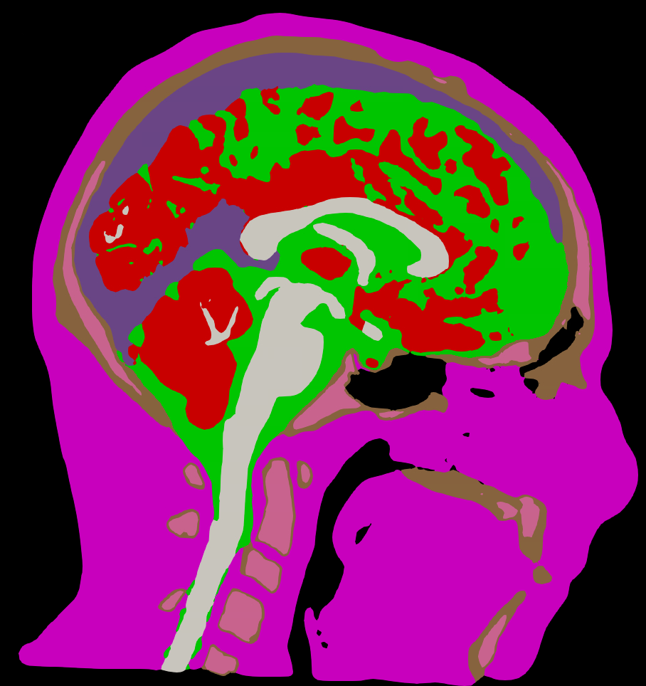
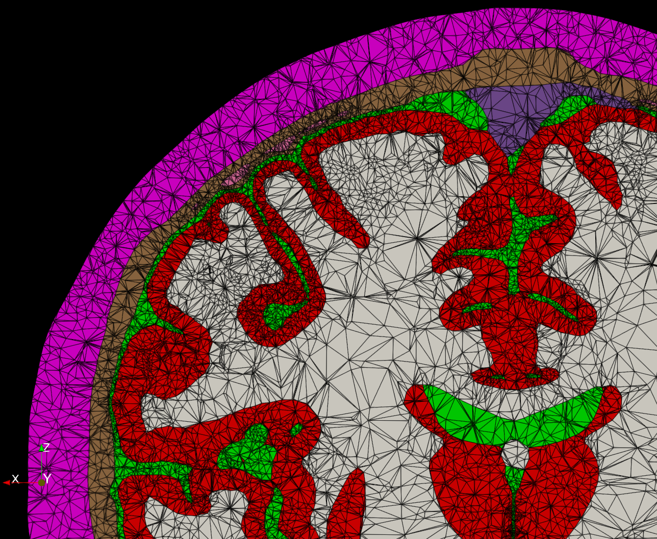
Figure. Different views of the headmodel showing edges projected on a slice (middle) and the full tetrahedral elements (bottom).

Converting EEG electrode locations to SimNIBS readable format

Next we need to prepare the electrodes. This means (1) aligning them with the MR image and (2) converting the result to a format which SimNIBS can read. We use the same template montage as is used in the above-mentioned FEM tutorial.

We start by aligning the electrodes to the MRI (and therefore also the headmodel). We will do this by matching the fiducials in the template montage (included in the template file) to the corresponding positions in the MRI (i.e., the target positions below which was manually identified on the MRI). Note that we set the channel type of the first three positions to fiducial as they correspond to LPA, RPA, and nasion, respectively. We do this so that they will be ignored by SimNIBS when converting the montage to CSV (as SimNIBS will only include channels with chantype eeg). We use method = 'template' in order to estimate a global rescaling parameter as well as translations and rotations.

% matlab
elec = ft_read_sens('standard_1020.elc');
[elec.chantype{1:3}] = deal('fiducial'); % these channels will be ignored by SimNIBS

cfg = [];
cfg.method = 'template';
cfg.warp = 'globalrescale'; % rigid-body plus global scaling
cfg.target.pos(1,:) = [-0.49 79.22 -26.95];
cfg.target.pos(2,:) = [-73.92 -27.38 -29.19];
cfg.target.pos(3,:) = [73.36 -22.29 -32.94];
cfg.target.label = {'Nz', 'LPA', 'RPA'}; % match names in elec.label
elec = ft_electroderealign(cfg, elec);

save elec.mat elec

disp(elec)

which should output something like

warping electrodes to average template... mean distance prior to warping 19.449876, after warping 4.452889
the call to "ft_electroderealign" took 1 seconds and required the additional allocation of an estimated 1 MB
          chanpos: [97×3 double]
         chantype: {97×1 cell}
         chanunit: {97×1 cell}
          elecpos: [97×3 double]
    globalrescale: [1.2003 -4.7868 10.2257 -2.9017 1.1005 2.3206 0.8726]
            label: {97×1 cell}
             type: 'eeg1010'
             unit: 'mm'
              cfg: [1×1 struct]

We can check the coregistration by loading the head mesh and plotting it together with the electrodes

% matlab
mesh = ft_read_headshape('m2m_Subject01/Subject01.msh');

figure;
hold on;
ft_plot_mesh(mesh,'surfaceonly','yes','vertexcolor', 'none', ...
    'edgecolor','none','facecolor','skin');
camlight;
ft_plot_sens(elec,'elecshape','sphere');
view(150, 26);
hold off;

Which should look something like the image below. As we are fitting template positions, the fit is not perfect.

Figure. Electrodes aligned with headmodel.

Next, we will use the function prepare_eeg_montage provided by SimNIBS to write the electrode information to a CSV file. This function assumes that the electrode structure is represented in the default FieldTrip format (as printed above). It reads a MAT file and assumes that it contains a variable elec describing the electrode montage. Now convert the montage to CSV

# shell
prepare_eeg_montage fieldtrip elec.csv elec.mat

This creates elec.csv. (Actually, we only require the fields elecpos, chanunit, chantype, and label to be present in the electrode structure.)

Running the FEM simulation

Now we are ready to actually run the simulation. This is the step where we do the actual forward calculations.

SimNIBS supports two solvers, PETSc (default) and PARDISO. The latter requires more memory than the former (16 GB or more) but is typically much faster, particularly for many electrodes. Here, we will use PETSc but feel free to try out the --pardiso option which will use the PARDISO solver. Using the PETSc solver, expect about 15 minutes to run the simulations.

# shell
prepare_tdcs_leadfield Subject01 elec.csv -s 10000

The subsampling flag, -s, sets the number of vertices (per hemisphere) where we want to compute the solution. (The original cortical surfaces produced by SimNIBS contain about 100,000 vertices per hemisphere.) These are selected by even subsampling over the whole surface. By default, we model electrodes as points, however, by using --mesh_electrodes, it is possible to mesh the electrodes onto the head model. Currently, electrodes are modeled as rings with a diameter of 10 mm and thickness of 4 mm. In our experiments, we have not found substantial effects of meshing electrodes, hence we omit this. By default, the results are stored in a directory called fem_Subject01.

To visualize the headmodel along with the electrodes projected on the skin surface (which is what we use in the simulations), we can use gmsh (which is included with SimNIBS)

gmsh m2m_Subject01/Subject01.msh -merge fem_Subject01/Subject01_electrodes_elec_proj.geo

(To show the electrode positions, tick the box under post-processing in the pane on the left-hand side.) Compare these with the positions before projection in the previous section.

Figure. Electrodes aligned and projected on headmodel.

Calculating the final forward model and exporting to FieldTrip

The final step is to prepare the EEG forward solution from the previous TDCS leadfield simulation. We do this by executing

# shell
prepare_eeg_forward fieldtrip Subject01 fem_Subject01/Subject01_leadfield_elec.hdf5

which will write three MAT files (to fem_Subject01) with the following endings and content

• -fwd.mat the forward solution (leadfield matrix).
• -src.mat the source space.

Let us load these into MATLAB

% matlab
load fem_Subject01/Subject01_leadfield_elec_subsampling-10000-fwd.mat;
load fem_Subject01/Subject01_leadfield_elec_subsampling-10000-src.mat;

and see what they contain

% matlab
>> fwd

fwd =

struct with fields:

                pos: [20000×3 double]
             inside: [20000×1 logical]
               unit: 'mm'
          leadfield: {1×20000 cell}
              label: {94×1 cell}
    leadfielddimord: '{pos}_chan_ori'
                cfg: 'Created by SimNIBS 4.0.1'

>> src

src =

struct with fields:
                    pos: [20000×3 double]
                    tri: [39992×3 int32]
                   unit: 'mm'
                 inside: [20000×1 logical]
         brainstructure: [1×20000 int64]
    brainstructurelabel: {'CORTEX_LEFT'  'CORTEX_RIGHT'}
                normals: [20000×3 double]

You should be able to use fwd as if it had been obtained from ft_prepare_leadfield and src as if obtained from ft_prepare_sourcemodel (with method = 'basedoncortex'), e.g., something like

% matlab
cfg = [];
cfg.sourcemodel = src;
cfg.sourcemodel.leadfield = fwd;
% cfg.method = ;
% source = ft_sourceanalysis(cfg, );

Work in progress

Source model

It would be nice to include options to write out the transfer matrix so that the results can be used with other source models, e.g., from DUNEuro. The source model is described in the reference at the top of this page.

Conductivities

It is currently not possible to specify the conductivities through this interface. Consequently, all simulations will use the default conductivities in SimNIBS.