Speeding up your analysis using distributed computing with qsub
If you are new to FieldTrip, we recommend that you skip this tutorial for now. You can read the introduction tutorial and then move on with the tutorials on preprocessing. Once you get the hang of it, you can return to this tutorial which is more on the technical and coding aspects.
Introduction
Many times you are faced with the analysis of multiple subjects and experimental conditions, or with the analysis of your data using multiple analysis parameters (e.g., frequency bands). Parallel computing in MATLAB can help you to speed up these types of analysis.
Note that this is usually referred to as distributed computing if you are submitting multiple independent computations to multiple computers. The term parallel computing is usually reserved for multiple CPUs or computers working simultaneously at the same problem that requires constant sharing of small snippets of data between the CPUs. Since the analyses of multiple subjects are done independently of each other, we call it distributed computing.
This tutorial describes two approaches for distributing the analysis of multiple subjects and conditions. The data used in this example is the same as in the tutorial scripts: 151-channel MEG was recorded in 4 subjects, and in each dataset there are three experimental conditions (FC, FIC, IC). Both approaches rely on the qsubcellfun function which applies a given function to each element of a cell-array. The function execution is done in parallel on the Torque batch queue system.
After this tutorial you should be able to execute your multi-subject analysis in parallel and design analysis scripts that allow for easy parallelization, either over subjects or over parameters used in the analysis.
In this tutorial we use the qsub toolbox that is released along with FieldTrip. There are alternative methods for distributed computing, such as the MATLAB Parallel Computing toolbox (e.g., using parfor or batch) or with the peer-to-peer toolbox (also included with FieldTrip). More general information about the different approaches for distributed processing in MATLAB can be found in the frequently asked questions.
Background
The qsub distributed computing toolbox was implemented with FieldTrip (and SPM) in mind. At the moment however, FieldTrip itself does not yet make use of distributed computing, i.e. FieldTrip functions do not automatically distribute the workload. We are of course planning to make that possible, i.e. that a single cfg.parallel=’yes’ option will automatically distribute the computational load over all available nodes.
At the moment the only way of distributing the workload over multiple nodes requires that you adapt your scripts. The easiest is to distribute the workload of the analysis of multiple subjects and conditions over multiple nodes.
Procedure
To distribute your processes and to speed up your analyses, we provide two examples. The first example script will show you how to use basic FieldTrip functions for the distribution. Using the basic FieldTrip functions in a memory efficient manner requires that you save the intermediate data of each step to disk, and that you load it upon the next (parallel) step in the analysis.
If you prefer not to store all intermediate results, or if you want to have more control over other aspects of the parallel execution, you can provide your own functions that are executed in parallel. This is demonstrated in the second example script.
The distributed operations of FieldTrip functions in this example require the original MEG datasets for the four subjects, which are available from
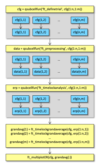
Example 1: using only FieldTrip functions in distributed computing
This example script demonstrates how to run basic FieldTrip functions in parallel. The idea is schematically depicted in the following figure.
subjectlist = {
'Subject01.ds'
'Subject02.ds'
'Subject03.ds'
'Subject04.ds'
};
conditionlist = {
'FC'
'FIC'
'IC'
};
triggercode = [
9
3
5
];
% start with a new and empty configuration
cfg = {};
for subj=1:4
for cond=1:3
cfg{subj,cond} = [];
cfg{subj,cond}.dataset = subjectlist{subj};
cfg{subj,cond}.trialdef.prestim = 1;
cfg{subj,cond}.trialdef.poststim = 2;
cfg{subj,cond}.trialdef.eventtype = 'backpanel trigger';
cfg{subj,cond}.trialdef.eventvalue = triggercode(cond);
end
end
cfg = qsubcellfun(@ft_definetrial, cfg, 'memreq', 4*1024^3, 'timreq', 10*60);
% this extends the previous configuration
for subj=1:4
for cond=1:3
cfg{subj,cond}.channel = {'MEG', '-MLP31', '-MLO12'};
cfg{subj,cond}.demean = 'yes';
cfg{subj,cond}.baselinewindow = [-0.2 0];
cfg{subj,cond}.lpfilter = 'yes';
cfg{subj,cond}.lpfreq = 35;
end
end
data = qsubcellfun(@ft_preprocessing, cfg, 'memreq', 4*1024^3, 'timreq', 10*60);
% start with a new and empty configuration
cfg = {};
for subj=1:4
for cond=1:3
% timelockanalysis does not require any non-default settings
cfg{subj,cond} = [];
end
end
timelock = qsubcellfun(@ft_timelockanalysis, cfg, data, 'memreq', 4*1024^3, 'timreq', 10*60);
% from here on we won't process the data in parallel any more
% average each condition over all subjects
cfg = [];
avgFC = ft_timelockgrandaverage(cfg, timelock{:,1});
avgFIC = ft_timelockgrandaverage(cfg, timelock{:,2});
avgIC = ft_timelockgrandaverage(cfg, timelock{:,3});
cfg = [];
cfg.layout = 'CTF151_helmet.mat';
ft_multiplotER(cfg, avgFC, avgFIC, avgIC);
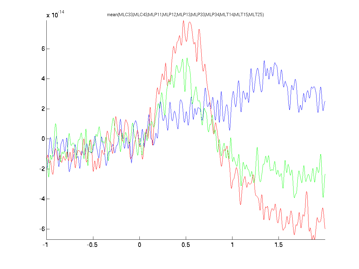
cfg = [];
cfg.channel = {'MLC33', 'MLC43', 'MLP11', 'MLP12', 'MLP13', 'MLP33', 'MLP34', 'MLT14', 'MLT15', 'MLT25'}
ft_singleplotER(cfg, avgFC, avgFIC, avgIC);
In the code above all data is processed by the distributed computers and subsequently returned to the workspace of your desktop computer. The data can take quite a lot of RAM, which you can check like this.
>> whos
  Name               Size                 Bytes  Class     Attributes

  conditionlist      3x1                    350  cell
  subjectlist        4x1                    544  cell
  triggercode        3x1                     24  double
  cfg                4x3                9732384  cell
  data               4x3             1203237420  cell
  timelock           4x3               65515200  cell
  ...
Instead of returning the 12 variables for the different subjects and conditions all to your workspace, you can also use the cfg.inputfile and cfg.outputfile options to have the distributed computers read/write the data to/from disk. For example the section on ft_preprocessing and ft_timelockanalysis could be changed into
% ...

for subj=1:4
  for cond=1:3
    cfg{subj,cond}.channel              = {'MEG', '-MLP31', '-MLO12'};
    cfg{subj,cond}.demean               = 'yes';
    cfg{subj,cond}.baselinewindow       = [-0.2 0];
    cfg{subj,cond}.lpfilter             = 'yes';
    cfg{subj,cond}.lpfreq               = 35;
    cfg{subj,cond}.outputfile           = sprintf('subj%02d_cond%02d_raw.mat', subj, cond);
  end
end

% note that here we don't specify an output parameter
qsubcellfun(@ft_preprocessing, cfg);

cfg = {};

for subj=1:4
  for cond=1:3
    cfg{subj,cond}.inputfile  = sprintf('subj%02d_cond%02d_raw.mat', subj, cond);
    cfg{subj,cond}.outputfile = sprintf('subj%02d_cond%02d_avg.mat', subj, cond);
  end
end

% note that here we don't specify an output parameter
qsubcellfun(@ft_timelockanalysis, cfg);

% ...
Example 2: writing custom functions for distributed computing
This example script demonstrates how you can efficiently design your custom code for distributed computing.
subjectlist = {
  'Subject01.ds'
  'Subject02.ds'
  'Subject03.ds'
  'Subject04.ds'
  };

conditionlist = {
  'FC'
  'FIC'
  'IC'
  };

triggercode = [
  9
  3
  5
  ];

% start with a new and empty configuration
cfg1 = {};
cfg2 = {};
cfg3 = {};
cfg4 = {};
outputfile = {};

for subj=1:4
  for cond=1:3
    % this is for definetrial and preprocessing
    cfg1{subj,cond}                      = [];
    cfg1{subj,cond}.dataset              = subjectlist{subj};
    cfg1{subj,cond}.trialdef.prestim     = 1;
    cfg1{subj,cond}.trialdef.poststim    = 2;
    cfg1{subj,cond}.trialdef.eventtype   = 'backpanel trigger';
    cfg1{subj,cond}.trialdef.eventvalue  = triggercode(cond);
    cfg1{subj,cond}.channel              = {'MEG', '-MLP31', '-MLO12'};
    cfg1{subj,cond}.demean               = 'yes';
    cfg1{subj,cond}.baselinewindow       = [-0.2 0];
    cfg1{subj,cond}.lpfilter             = 'yes';
    cfg1{subj,cond}.lpfreq               = 35;

    % this is for timelockanalysis
    cfg2{subj,cond}                      = [];

    % this is for megplanar
    cfg3{subj,cond}                      = [];

    % this is for combineplanar
    cfg4{subj,cond}                      = [];

    % this defines the file that will contain the output
    outputfile{subj,cond} = sprintf('subj%02d_cond%02d_combined.mat', subj, cond);
  end
end

% note that the "preproc_timelock_planar" function is defined further down in this tutorial
qsubcellfun(@preproc_timelock_planar, cfg1, cfg2, cfg3, cfg4, outputfile);

% let's now load the individual subject data from the 12 .mat files and average each of them for subsequent plotting
timelock = {};
for subj=1:4
  for cond=1:3
    tmp = load(sprintf('subj%02d_cond%02d_combined.mat', subj, cond));
    timelock{subj,cond} = tmp.combined;
    clear tmp
  end
end

cfg = [];
avgFC  = ft_timelockanalysis(cfg, timelock{:,1));
avgFIC = ft_timelockanalysis(cfg, timelock{:,2));
avgIC  = ft_timelockanalysis(cfg, timelock{:,3));

cfg = [];
cfg.layout = 'CTF151_helmet.mat';
ft_multiplotER(cfg, avgFC, avgFIC, avgIC)
This way you can distribute your custom function (e.g., see below) along with the input and output parameters.
function preproc_timelock_planar(cfg1, cfg2, cfg3, cfg4, outputfile)

cfg1 = ft_definetrial(cfg1);
data = ft_preprocessing(cfg1);

timelock = ft_timelockanalysis(cfg2, data);
clear data

planar = ft_megplanar(cfg3, timelock);
clear timelock

combined = ft_combineplanar(cfg4, planar);
clear planar

save(outputfile, 'combined');
clear combined
Summary and suggested further reading
This tutorial covered how to distribute your computations/workload over multiple computers in a cluster that uses the Torque or SGE batch queue system. In our example, we have performed a relatively simple timelock analysis to compute event-related fields, but one can imagine that it does not need many adjustments to distribute any other type of analysis. Using the configuration demonstrated in Example 2, you can distribute any form of analysis.
FAQs related to issues in this tutorial:
- How to compile MATLAB code into stand-alone executables?
- How to get started with distributed computing using qsub?
- What are the different approaches I can take for distributed computing?