Channel and source analysis of mouse EEG
Introduction
This tutorial describes the processing of mouse EEG data. Although the mouse EEG data as demonstrated here is not recorded intracranial (i.e., inside the skull), the recording is invasive and as such more comparable to ECoG than to normal scalp EEG. The implantation and recording method for the data in this tutorial is explained in this video tutorial, which also points to information on optical stimulation of the mouse brain through an optical fiber.
This tutorial deals with preprocessing, computing ERPs, time-frequency analysis, and visualization of channel-level data. Furthermore, it deals with reading and processing anatomical data, the coregistration with EEG electrodes, and the construction of a volume conduction model and source model. Finally, the EEG data is source reconstructed.
To learn how to process EEG data in more general, we suggest you check the tutorial on EEG preprocessing computing ERPs. More information on the processing of human intracranial data, including the coregistration and electrode localization, can be found in the human ECoG and sEEG tutorial.
Background
The purpose of the study described here is to use EEG combined with optogenetic stimulation (so called opto-EEG) for studying sensorimotor integration. Sensorimotor integration is a neurological process dealing with somatosensation inputs into motor outputs in an effective way. Numerous studies have shown the direct signal pathways within somatosensor-motor circuits, however little is known how the tactile sensations with different stimulation frequency are processed from somatosensory to motor cortex in order to react appropriately to different types of stimulation.
Transgenic mice were used for the study (Thy1-ChR2-EYFP, B6 mice, 12 weeks; body weight 27 g, malehttp://jaxmice.jax.org/strain/007615.html). For implantation of electrodes on the skull and sensory thalamus (VPM; 1.82 mm posterior, 1.5 mm lateral and 3.7 mm ventral to bregma), mice were anesthetized (ketamine/xylazine cocktail, 120 and 6 mg/kg, respectively) and then positioned in a stereotaxic apparatus.
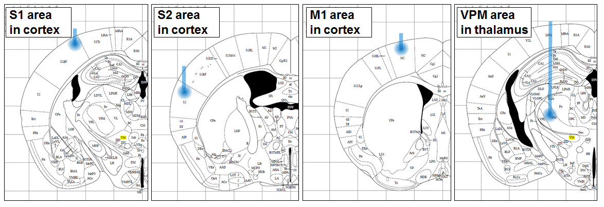
For optogenetic stimulation, a semiconductor laser was used (USA & BCL-040-445; 445 nm wavelength and 40 mW/mm2 maximum output power; CrystaLaser LLC., Reno, NV, USA) that was gated using a pulse generator (575 digital delay, Berkeley Nucleonics Corp., Berkeley, CA, USA). Blue light from the laser was guided to the brain using an optic fiber with clad/core diameters of 125 mm and 3.4 mm, respectively (P1-405A-FC-5; Thorlabs Inc., Newton, NJ, USA). The light intensity from the tip of optical fiber was approximately 2 mW/mm2 measured by integrating sphere coupled to spectrometer (BLUE-Wave-VIS2/IC2/IRRAD-CAL, Stellar-Net Inc., Tampa, FL, USA). Various pulse trains with a 20 ms pulse width were delivered in four different cortical regions (somatosensory cortices, primary motor cortex, and sensory thalamus marked as S1, S2, M1, and VPM in below figure, respectively).
Figure: Regions of interest.
Peripheral sensation was mimicked by direct optogenetic stimulation of S1, S2, M1 and sensory thalamus and concurrently recorded the frequency dependent responses (1, 10, 20, 30, 40 and 50 Hz) with a depth electrode in the region of the optode (i.e. S1, S2, M1 and thalamus). Furthermore, EEG was recorded on the surface of the skull using a high-density micro electrode array. Two electrodes in the most anterior region were allocated as the reference and ground. The signals from the brain were recorded both by high-density micro electrode array (EEG = 38 channels, plus ground and reference, so 40 electrodes) and from an sharp-tipped implanted electrode as the local field potential (single channel). The EEG and LFP were acquired with an analog amplifier (Synamp, Neuroscan, USA) with a sampling frequency of 2000 Hz.
The dataset used in this tutorial
The data for this tutorial can be downloaded from our download server.
Procedure
The procedure consists of the following steps:
- preprocessing
- define trials
- reading and filtering
- checking for artifacts
- rereferencing
- time-locked averaging
- making a channel layout
- deal with differences in animal size
- channel-level analysis - ERPs
- channel-level analysis - TFRs
- anatomical processing
- read the anatomical MRI data
- coregister it
- read the atlas data
- coregister it
- prepare the headmodel
- make segmentation of brain tissue
- make mesh of boundaries
- make BEM volume conduction model
- specification of electrodes
- deal with differences in animal size
- make the source model and leadfields
- do source reconstruction
- visualize source reconstruction
- look up source results in atlas
Preprocessing
Define trials
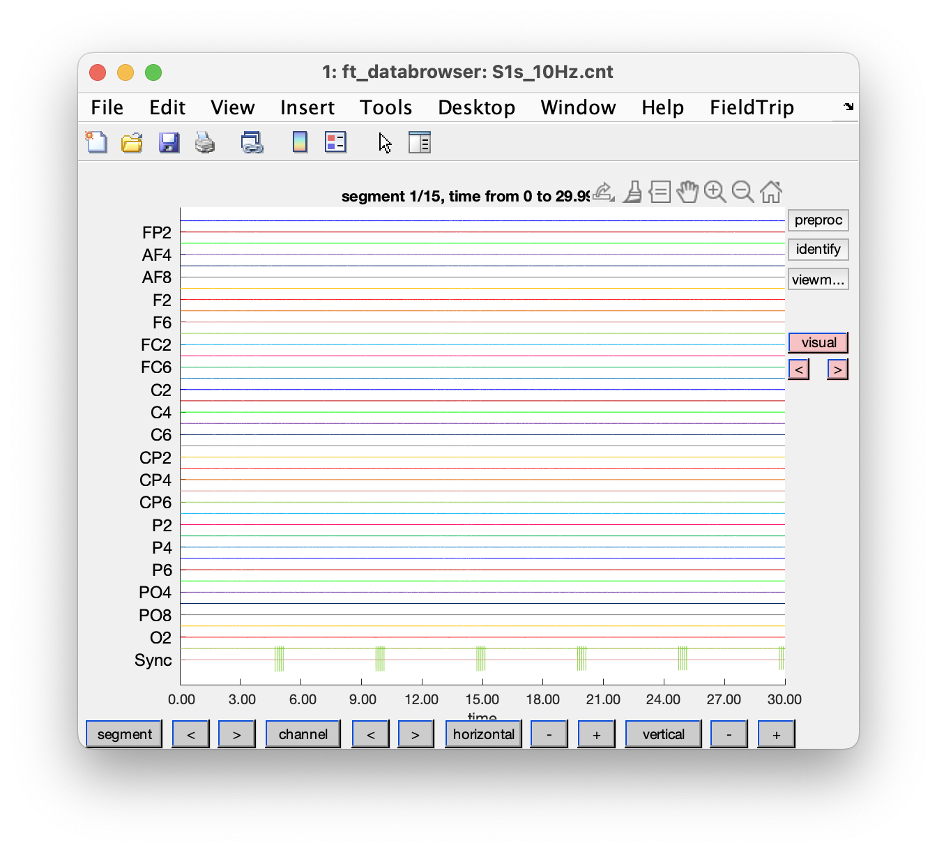
We start with a visual inspection of the data.
cfg = [];
cfg.dataset = 'S1s_10Hz.cnt';
cfg.viewmode = 'vertical';
cfg.blocksize = 30; % show 30 seconds per page
cfg = ft_databrowser(cfg);
Figure: Exploring the data on disk with ft_databrowser.
Using ft_definetrial and ft_preprocessing we define, read and preprocess the data segments of interest. Trials are specified by their begin and end sample in the data file and each trial has an offset that defines where the relative t=0 point (usually the point of the optogenetic stimulus-trigger) is for that trial.
The dataset used here does not include digital trigger information. To record the timing of stimulation, an analog input channel ‘HL1’ was used to record TTL triggers. We use a customized function and the cfg.trialfun='mousetrialfun' option to define the segments. The trial function results in the output of ft_definetrial in a cfg.trl Nx3 array that contains the begin- and endsample, and the trigger offset of each trial relative to the beginning of the raw data on disk.
function trl = mousetrialfun(cfg)

% this function requires the following fields to be specified
% cfg.dataset
% cfg.trialdef.threshold
% cfg.trialdef.prestim
% cfg.trialdef.poststim

hdr = ft_read_header(cfg.dataset);
trigchan = find(strcmp(hdr.label, 'HL1'));
trigger_data = ft_read_data(cfg.dataset, 'chanindx', trigchan); % read trigger data
trigger_data = -trigger_data; % flip sign
trigger_data = trigger_data - median(trigger_data); % shift

if isfield(cfg, 'trialdef') && isfield(cfg.trialdef, 'threshold')
  trigger_threshold = cfg.trialdef.threshold;
else
  trigger_threshold = 0.5*max(trigger_data);
end

% give some feedback
figure
plot(trigger_data, 'b')
hold on
plot(trigger_threshold*ones(size(trigger_data)), 'g')

stim_duration = cfg.trialdef.prestim  * hdr.Fs; % number of samples
rest_duration = cfg.trialdef.poststim * hdr.Fs; % number of samples

% extracts, trigger timing ------------------------------------------------
data1 = find(abs(trigger_data) > trigger_threshold);      % exceed threshold
data2 = find(data1-[0,data1(1,1:end-1)] > rest_duration); % exceed 'rest_duration'
idx = data1(data2);
clear data1 data2

trigger_event(1,:) = idx;
clear idx

% give some additional feedback
plot(trigger_event(1,:), trigger_threshold, 'rx')

% extracts, trigger contents ----------------------------------------------
for tr = 1:size(trigger_event,2)
  temp_data = abs(trigger_data(trigger_event(1,tr):trigger_event(1,tr)+stim_duration-1));
  idx = find_cross(temp_data, trigger_threshold, 'down'); clear temp_data
  trigger_event(2,tr) = size(find(idx == 1),2) / (stim_duration / hdr.Fs);
end

trl       = [trigger_event(1, :) - stim_duration+1; trigger_event(1, :) + rest_duration]';
trl(:, 3) = zeros(size(trl, 1), 1);

function idx = find_cross(data, thr, type)
% find peaks.
% data = 1 by n vector.
% thr = the crossing point.
% type = 'both', 'up', 'down'.
% default type: 'both'.

if size(data,1) > 1
  data = data.';
  if size(data,2) > 1
    error('data must be vector form')
  end
end

% up crossing
tidx1 = zeros(1,size(data,2)-1);
tidx2 = zeros(1,size(data,2)-1);
idx1 = zeros(1,size(data,2)-1);
tidx1(data(1,1:end-1) <= thr) = 1;
tidx2(data(1,2:end) > thr) = 1;
idx1(tidx1 + tidx2 == 2) = 1; clear tidx1 tidx2

% down crossing
tidx1 = zeros(1,size(data,2)-1);
tidx2 = zeros(1,size(data,2)-1);
idx2 = zeros(1,size(data,2)-1);
tidx1(data(1,1:end-1) >= thr) = 1;
tidx2(data(1,2:end) < thr) = 1;
idx2(tidx1 + tidx2 == 2) = 1; clear tidx1 tidx2

% both
idx0 = zeros(1,size(data,2)-1);
idx0(idx1 + idx2 > 0) = 1;

if nargin == 2
  idx = idx0;
elseif nargin == 3
  if strcmpi(type,'both')
    idx = idx0;
  elseif strcmpi(type,'up')
    idx = idx1;
  elseif strcmpi(type,'down')
    idx = idx2;
  end
end
Using this trial function, we can call ft_definetrial to find the trials or segments of interest.
cfg = [];
cfg.dataset  = 'S1s_10Hz.cnt';
cfg.trialfun = 'mousetrialfun'; % see above
cfg.trialdef.threshold = 2e6;
cfg.trialdef.prestim    = 1; % in seconds
cfg.trialdef.poststim   = 2; % in seconds
cfg = ft_definetrial(cfg);
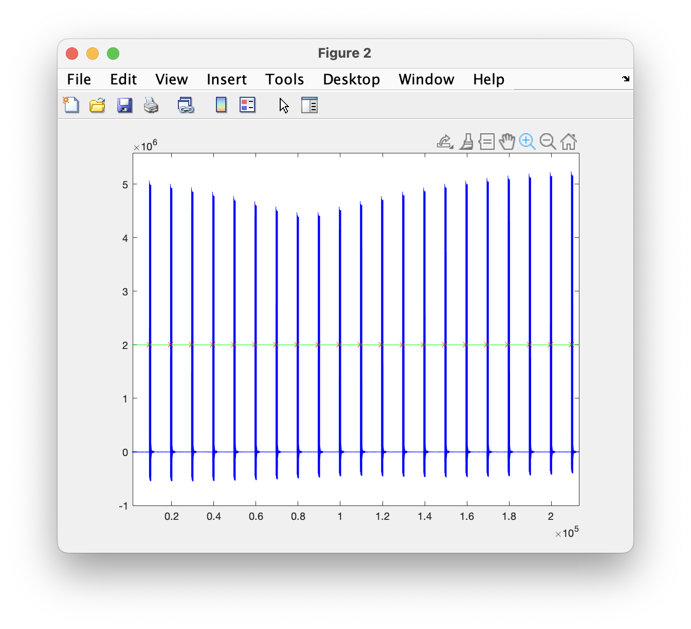
You will see that the trial function produces a figure, which can be used to check the pulses, whether the threshold was appropriate, and whether the stimulation onsets are properly detected.
Figure: Feedback from mousetrialfun after zooming in.
The segments of interest are specified by their begin- and endsample and by the offset that specifies the timing relative to the data segment. The offset is -2000, indicating that sample 2000 in every trial is considered as time t=0.
>> cfg.trl

ans =
    7447       13446       -2000
   17447       23446       -2000
   27447       33446       -2000
   37447       43446       -2000
   47447       53446       -2000
   57447       63446       -2000
   67447       73446       -2000
   ...
Reading and filtering
After the segments of interest have been specified as cfg.trl, we read them from disk into memory using ft_preprocessing. Note that the same function could also have been used to read the data continuously (as a single long segment). At this step we also specify other preprocessing options such as the filter settings.
cfg.channel   = 'all';
cfg.baseline  = [-0.30, -0.05];
cfg.demean    = 'yes';
cfg.bsfilter  = 'yes';
cfg.bsfreq    = [59 61]
cfg.lpfilter  = 'yes';
cfg.lpfreq    = 100;
data          = ft_preprocessing(cfg);
The output of ft_preprocessing is a structure which has the following fields:
data =
           hdr: [1x1 struct]
         label: {39x1 cell}
          time: {1x88 cell}
         trial: {1x88 cell}
       fsample: 2000
    sampleinfo: [88x2 double]
           cfg: [1x1 struct]
In data.sampleinfo you can recognize the begin and endsample of each trial: these are copied over from the 1st and 2nd column of cfg.trl. The offset in the 3rd column has been used to make an individual time axis data.time for each trial.
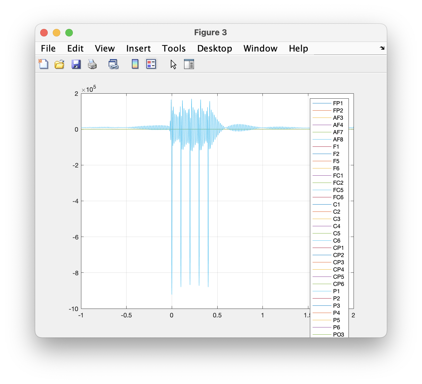
We can plot all channels for a single trial using standard MATLAB code.
figure
plot(data.time{1}, data.trial{1});
legend(data.label);
grid on
Figure: Plot of a single trial.
Checking for artifacts
Using ft_databrowser we can do a visual inspection of the data in each trial and check for artefacts.
cfg = [];
cfg.viewmode = 'butterfly';
cfg = ft_databrowser(cfg, data);
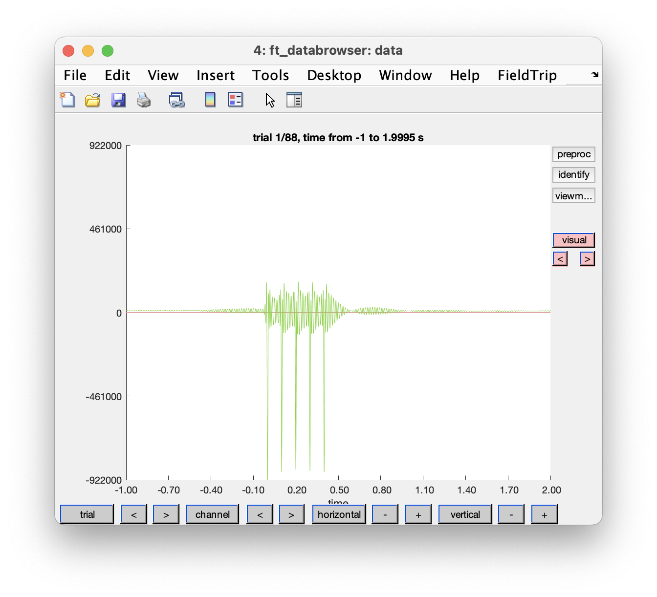
Figure: Single trial with ft_databrowser in butterfly mode.
The 41th channel with label ‘HL1’ contains the analog TTL trigger, which is of much larger amplitude than all other channels. We can exclude it in the GUI by clicking the “channel” button and removing it or by using the following code:
cfg = [];
cfg.viewmode = 'vertical';
cfg.channel = {'all', '-HL1'};
cfg = ft_databrowser(cfg, data);
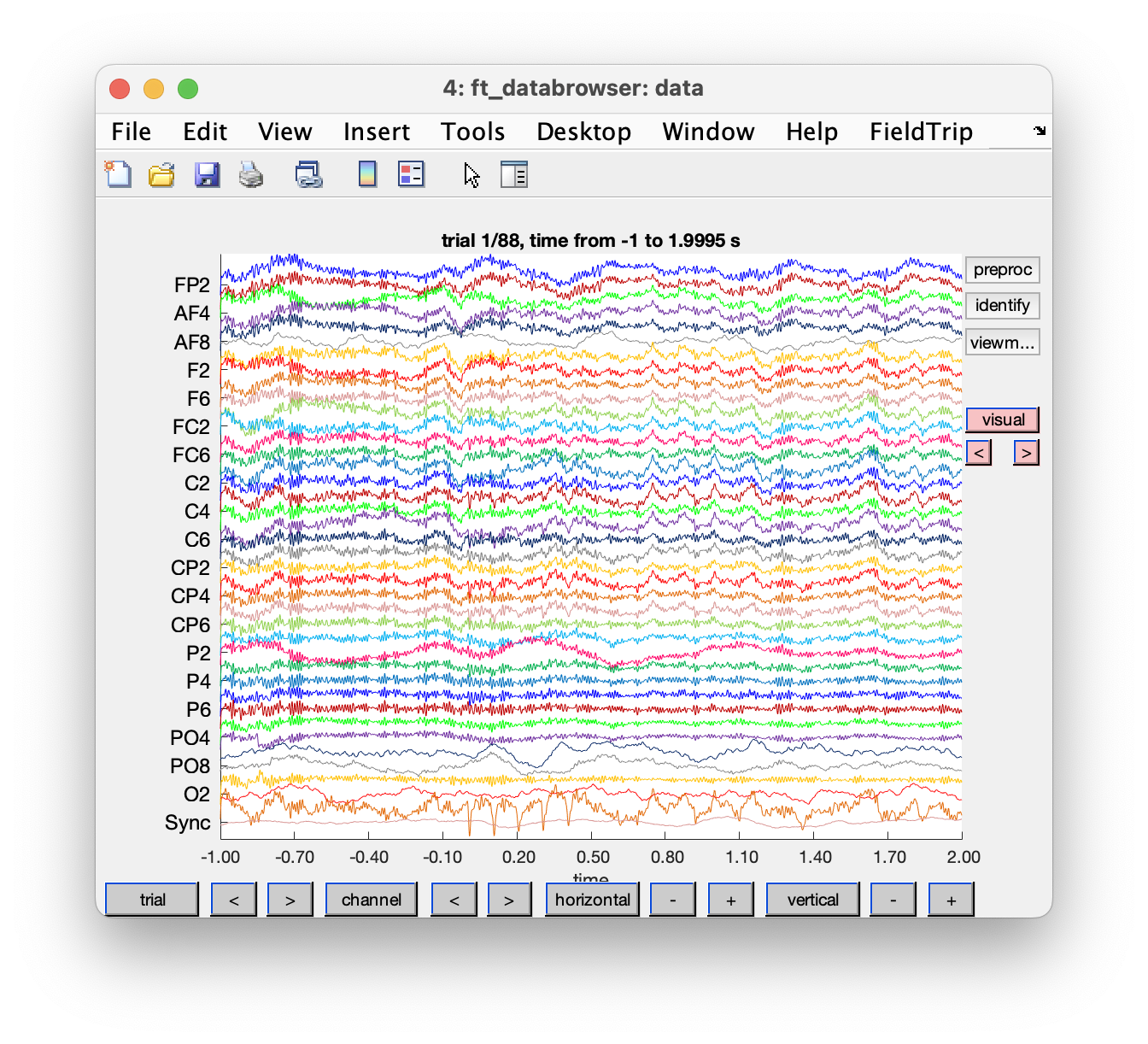
Some channels show a much lower noise level than others (e.g., AF8). This might be due to differences in the electrode-skull impedance.
Figure: Single trial with ft_databrowser in vertical mode.
If you have selected visual artifacts, the output cfg of ft_databrowser will contain those artifacts. You could call ft_rejectartifact to remove the artifacts.
Rereferencing
The two most frontal electrodes in the grid, just anterior of the Fp1 and the Fp2 electrode, were used during the recording as the ground and reference. For the subsequent analyses we rereference the data to a common average over all electrodes.
cfg            = [];
cfg.reref      = 'yes';
cfg.channel    = {'all', '-VPM', '-Sync', '-HL1'};  % we don't want to re-reference these
cfg.refchannel = {'FP1';'FP2';...
                  'AF3';'AF4';'AF7';'AF8';...
                  'F1';'F2';'F5';'F6';...
                  'FC1';'FC2';'FC5';'FC6';...
                  'C1';'C2';'C3';'C4';'C5';'C6';...
                  'CP1';'CP2';'CP3';'CP4';'CP5';'CP6';...
                  'P1';'P2';'P3';'P4';'P5';'P6';...
                  'PO3';'PO4';'PO7';'PO8';...
                  'O1';'O2'};
data_reref = ft_preprocessing(cfg, data);
We have now lost the LFP in the ‘VPM’ channel, since that should not be rereferenced to the common average reference. We can get it back from the original data and append it to the rereferenced EEG data.
cfg = [];
cfg.channel = 'VPM';
data_vmp = ft_selectdata(cfg, data);

cfg = [];
data_reref = ft_appenddata(cfg, data_reref, data_vmp);
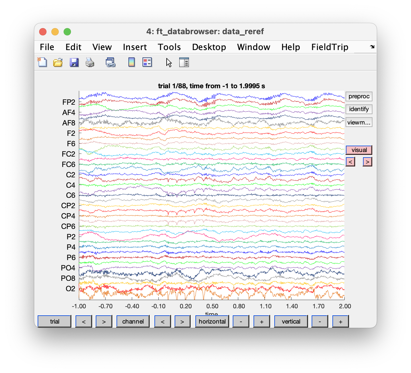
You can compare the original and re-referenced data using ft_databrowser.
cfg = [];
cfg.viewmode = 'vertical';
ft_databrowser(cfg, data_reref);
Figure: Single trial in ft_databrowser after re-referencing.
Making a channel layout for plotting
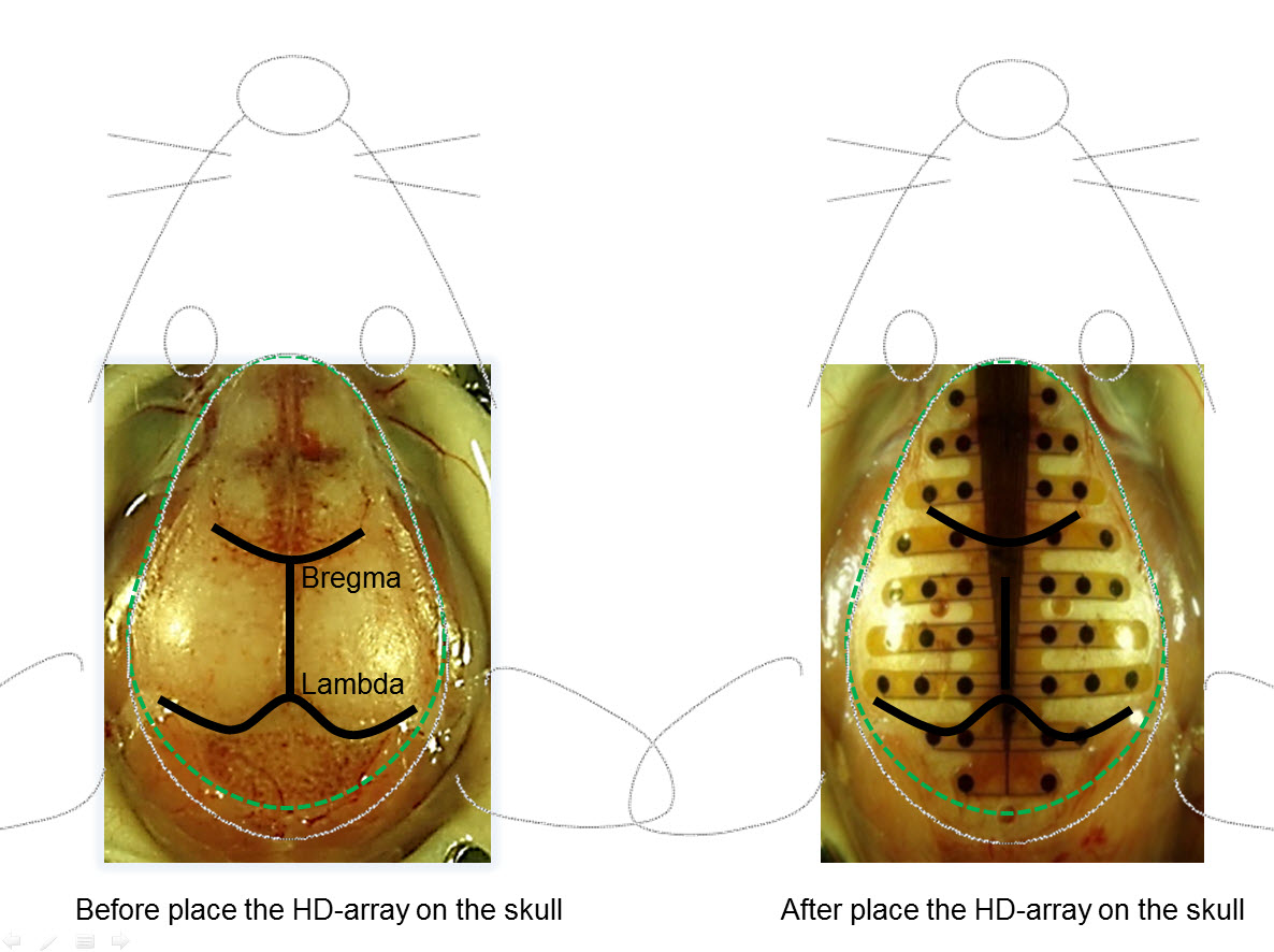
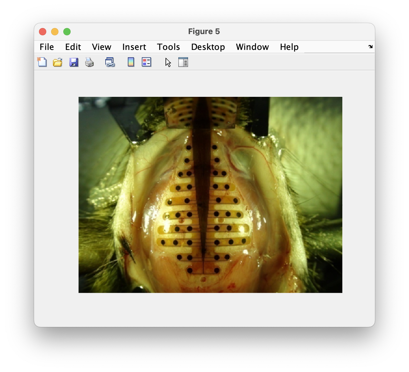
For 2D plotting of the channel data, FieldTrip makes use of so-called layouts. These layouts specify the location and size of each channel in the figure, and can include an outline (for example of the mouse head) and a mask to restrict the topographic interpolation for topoplots. The goal is to create a layout that combines the pre- and post- electrode placement photo, plus some anatomical features of the mouse head to make it easier recognizeable.
Figure: Outline of the desired image for the channel layout.
The bregma and lambda points are located along the anterio-posterior axis of the Paxinos coordinate system. The electrode array has been carefully aligned with the anterio-posterior axis between bregma and lambda points. As the coordinate system origin (0,0), the array was placed such that the bregma point is located in the middle of the 4th row of the electrode array.
For the layout of the EEG array, we start with a photo of the electrode arrangement taken from Lee et al. (2011) Journal of Visualized Experiments (video, pdf).
You can specify cfg.image in ft_prepare_layout and subsequently click on the location of each electrode. Note that you should click on the electrode positions in the right order and that you should skip the two most frontal electrodes, as those are the ground and reference and don’t have a corresponding channel.
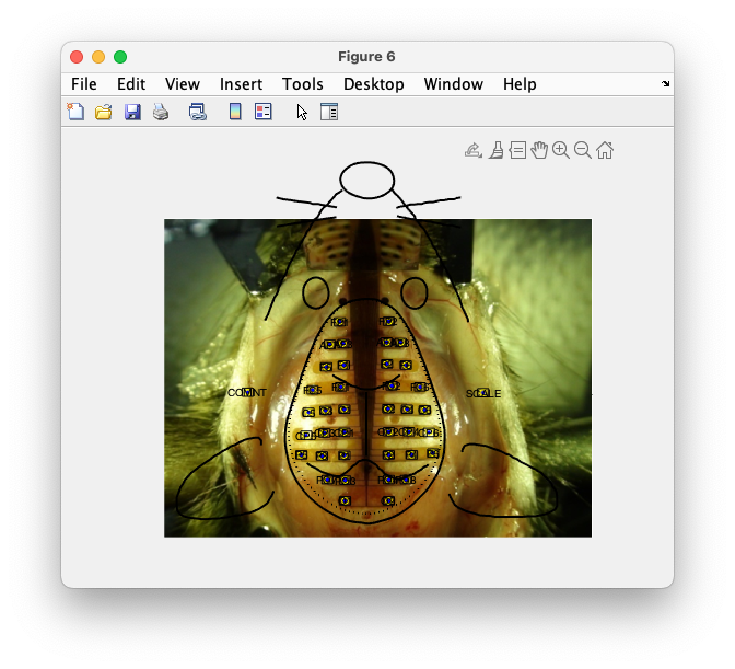
After specifying each electrode location, you’ll be asked to specify points that - when connected - form the outlines of the head. In human EEG the we would use a circle around the head as the outline, here we draw the eyes, the ears, and the nose with some whiskers. Furthermore we add lines representing other important landmarks that help to orient: in this case bregma and lambda. Besides the bold lines that specify the outline, we specify a mask for the topographic interpolation (dashed line).
cfg          = [];
cfg.image    = 'mouse_skull_with_HDEEG.png';
cfg.channel  = {'FP1' 'FP2' 'AF3' 'AF4' 'AF7' 'AF8' 'F1' 'F2' 'F5' 'F6' 'FC1' 'FC2' 'FC5' 'FC6' 'C1' 'C2' 'C3' 'C4' 'C5' 'C6' 'CP1' 'CP2' 'CP3' 'CP4' 'CP5' 'CP6' 'P1' 'P2' 'P3' 'P4' 'P5' 'P6' 'PO3' 'PO4' 'PO7' 'PO8' 'O1' 'O2'};
layout_pixels = ft_prepare_layout(cfg);
Figure: The background image in ft_prepare_layout.
For the purpose of this tutorial, making precise and detailed outlines of the eyes, nose, whiskers and ears are not necessary, but you should try to understand how you can add them and how they are represented in the layout structure.
After creating the layout, you should check that all channel labels match with the corresponding position. The channel order in layout.label should correspond to the sequence in which you clicked the electrodes. You will see that placeholders have been added for the comments (COMNT) and the scale (SCALE). You can repeatedly call ft_plot_layout for a visual inspection of the layout. Furthermore, you can add the original image as the background.
img = imread('mouse_skull_with_HDEEG.png');
img = flip(img, 1); % in combination with "axis xy"

figure
image(img);
axis xy % see "help axis" for the difference between "ij" and "xy"
ft_plot_layout(layout_pixels)
Figure: Plot of the 2D layout with the image.
A stereotactic ruler was used to determine the size of the specific mouse depicted in the photo; the distance between the bregma and lambda points on the skull was 4.2 mm. This number is used later to deal with animals with a different head size. We also identified the bregma and lambda points in the photographic image.
bregma = [343 252];
lambda = [343 130];
To make a calibrated layout in millimeters that matches the actual animal size, we want to get the bregma point precisely at the origin (0,0). We subtract the position of the bregma in the image from the position of all electrodes, outlines and masks. We furthermore want the distance between bregma and lambda to be 4.2 mm, hence we scale all positions by the ratio between the distance in pixels and millimeters.
layout_mm = layout_pixels;

shift = bregma;
layout_mm.pos = layout_mm.pos - repmat(shift, size(layout_mm.pos, 1), 1);
for i=1:numel(layout_mm.outline)
  layout_mm.outline{i} = layout_mm.outline{i} - repmat(shift, size(layout_mm.outline{1, i}, 1), 1);
end
for i=1:numel(layout_mm.mask)
  layout_mm.mask{i} = layout_mm.mask{i} - repmat(shift, size(layout_mm.mask{1, i}, 1), 1);
end

scale = 4.2/norm(bregma-lambda); % use the norm to compute the length of the vector
layout_mm.pos    = layout_mm.pos    * scale;
layout_mm.width  = layout_mm.width  * scale;
layout_mm.height = layout_mm.height * scale;
for i=1:numel(layout_mm.outline)
  layout_mm.outline{i} = layout_mm.outline{i} * scale;
end
for i=1:numel(layout_mm.mask)
  layout_mm.mask{i} = layout_mm.mask{i} * scale;
end
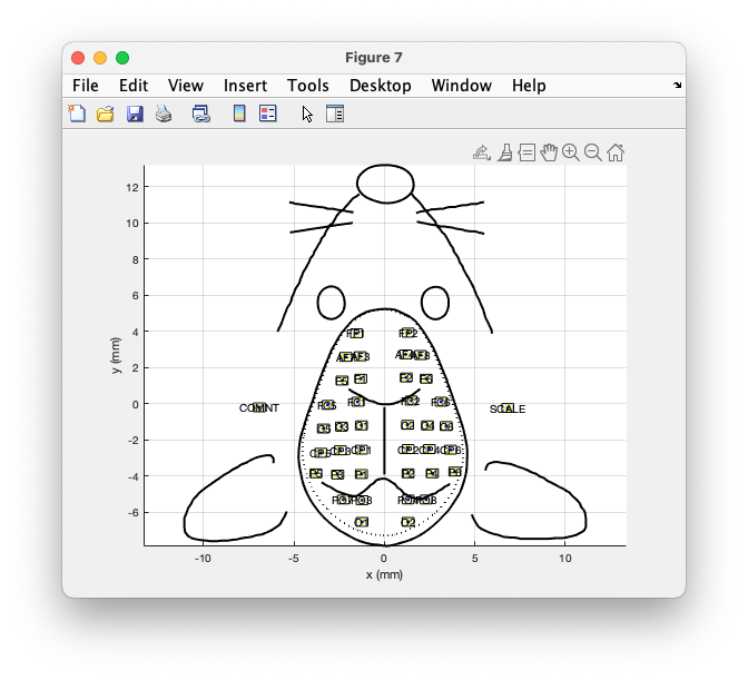
We plot it with the coordinate axes and a grid to confirm the calibration.
figure
ft_plot_layout(layout_mm)
axis on
grid on
xlabel('x (mm)')
ylabel('y (mm)')
Figure: Plot of the layout, calibrated in mm.
If you are satisfied with the result, you should save it to a MATLAB file. However, in the case of this specific tutorial you probably don’t want to overwrite the mat file that you have downloaded, but rather read that from disk and inspect it with ft_plot_layout.
if false
  save layout_pixels.mat layout_pixels
  save layout_mm.mat     layout_mm
else
  load layout_pixels.mat
  load layout_mm.mat
end
Deal with differences in animal size
Human heads differ in size, but the EEG caps also come in different sizes, for example ranging from 52 to 60 cm head circumference in 2cm steps. Furthermore, those EEG caps are slightly stretchable to have a tight but comfortable fit and to deal with the 2 cm range of the confection sizes. For the channel level plotting of human EEG we can therefore conveniently make use of template layouts that are the same for all participants.
The polyimide film from which the high-density mouse EEG array is made is not stretchable. Each mouse, however, has a different head size depending on its strain, age, weight and sex. To deal with the different sizes, we use a reference scale of 4.2 mm for the distance between bregma and lambda. If you have a smaller mouse, and consequently a relatively wider spaced EEG array for that specific mouse, you can scale the layout to accommodate this. The approach here to deal with differences in the mouse brain size is very comparable to the one adopted in the Talairach-Tournoux anatomical atlas of the human brain.
For example, let’s think about a case of targetting CA1 hippocampus which is (AP, ML, DV) = (-2, 1.5, -2) with respect to the bregma according to the mouse atlas. Each individual mouse has a different brain size. What we do is to measure the length between bregma to lambda, and if the length is 3.8 mm, we multiply the target distance by 38/42 = 0.9048. Hence the stereotaxic target for CA1 becomes (AP, ML, DV) = (-1.8095, 1.3571, -1.8095) and since the accuracy of the stereotaxic is 0.1 mm, the actual target becomes (-1.8, 1.4, -1.8). Note that some mouse research groups rescale only anterior posterior (AP) and according to them the target coordinate would be (-1.8, 1.5, -2).
The same scaling can be used for the high-density mouse EEG array. For example, for a mouse with a bregma-lambda distance of 3.8, you can do the following.
layout42 = layout_mm; % this was the reference animal
layout38 = [];        % start with an empty structure

ratio = 3.8/4.2;

layout38.pos    = layout42.pos;     % this remains the same
layout38.width  = layout42.width;   % this remains the same
layout38.height = layout42.height;  % this remains the same
layout38.label  = layout42.label;   % this remains the same
for i=1:numel(layout42.outline)
  layout38.outline{i} = layout42.outline{i} * ratio; % this gets scaled
end
for i=1:numel(layout42.mask)
  layout38.mask{i} = layout42.mask{i} * ratio; % this gets scaled
end

save layout42.mat layout42
save layout38.mat layout38
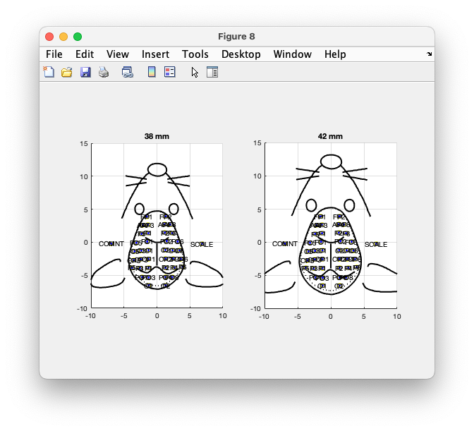
Again, to confirm your calibration:
figure

subplot(1,2,1)
title('38 mm')
ft_plot_layout(layout38)
axis on
axis([-10 10 -10 15])
grid on

subplot(1,2,2)
title('42 mm')
ft_plot_layout(layout42)
axis on
axis([-10 10 -10 15])
grid on
Figure: Plot of the layout for a 3.8 mm and 4.2 mm mouse.
In the mouse we can use histology as a a secondary confirmation procedure after recordings. The anatomical structure of mouse brain due not vary dramatically if the weight and/or the length between bregma and lambda are in the similar range, in the order of a few hundreds micrometer. Consequently, we seldom fail to hit a structure larger than a couple of hundreds micrometer. However, when we aim for a structure with a sharp shape with dimension smaller than a couple of hundreds micrometer, the chance of hitting that structure is considerably lower.
Channel level analysis - ERPs
The ERP time-locked to stimulus onset is computed by averaging the data over all trials.
cfg = [];
timelock = ft_timelockanalysis(cfg, data_reref);
We can again plot it with a standard MATLAB command.
figure
plot(timelock.time, timelock.avg);
legend(timelock.label);
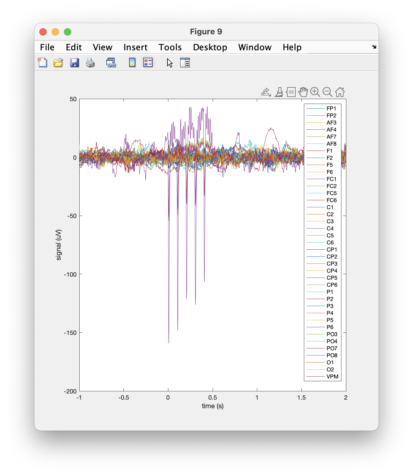
Figure: Plot of the ERP for all channels.
Looking at the figure legend, you can see that channel VPM shows a particularly large response to the stimulation. This makes sense, as it corresponds to the depth electrode that is inserted along with the optode, i.e. it records from the stimulated site.
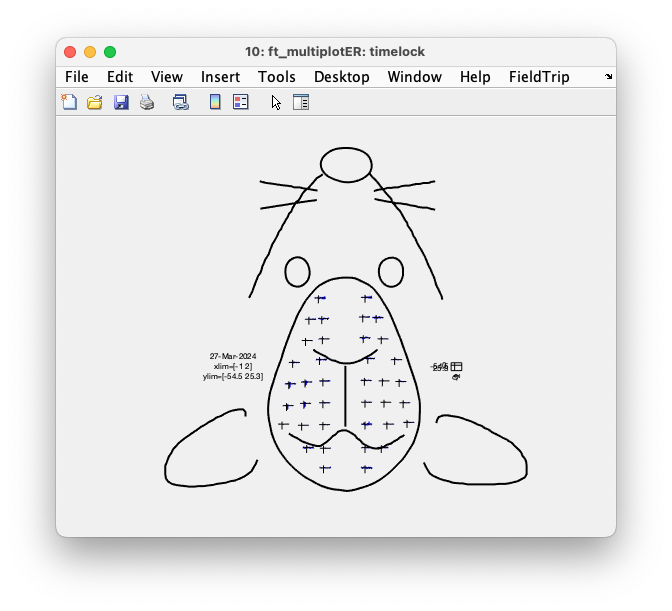
Rather than plotting all ERPs on top of each other, we can also plot them according to the channel layout that we constructed above. For that we use the function ft_multiplotER.
cfg             = [];
cfg.layout      = 'layout42.mat';  % from file
cfg.showoutline = 'yes';
cfg.interactive = 'yes';
ft_multiplotER(cfg, timelock);
Figure: Interactive plot of all channels using ft_multiplotER.
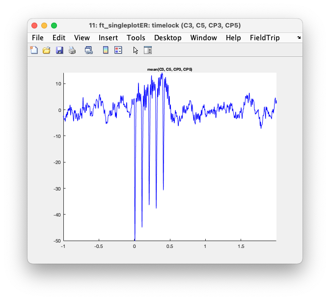
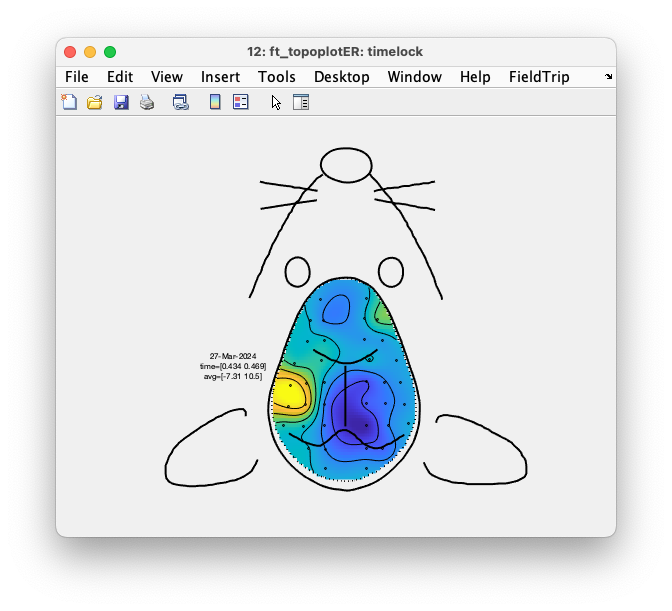
When you specify cfg.interactive = 'no' you can use the MATLAB zoom buttons. With cfg.interactive = 'yes' the zoom buttons don’t work properly, but you can make a selection of channels and click in the selection, which causes them to be averaged and displayed in a single plot. In the single plot, you can again make a selection of time, which is subsequently averaged (for all channels) and shown as the interpolated topographic distribution of the potential.
Figure: Interaction results in a ft_singleplotER figure.
Figure: Interaction results in a ft_topoplotER figure.
Channel level analysis - TFRs
This section describes how to calculate time-frequency representations using Hanning window.
% power spectrogram
cfg                   = [];
cfg.output            = 'pow';
cfg.method            = 'mtmconvol';
cfg.taper             = 'hanning';
cfg.foi               = 4:4:100;                         % frequencies of interest
cfg.t_ftimwin         = ones(length(cfg.foi),1)*0.250;   % 250 ms window
cfg.toi               = -1:0.01:3.0;                     % from -1 to 3 seconds in steps of 0.01
freq                  = ft_freqanalysis(cfg, data_reref);
The output of ft_freqanalysis is a structure which has the following fields:
freq =
    powspctrm: [39x25x401 double]
       dimord: 'chan_freq_time'
        label: {39x1 cell}
         freq: [4 8 12 16 20 24 ... 96 100]
         time: [-1 -0.9900 -0.9800 -0.9700 ... 2.9900 3.0000]
          cfg: [1x1 struct]
The field freq.powspctrm contains the power for each of the 39 channels, for each of the 401 timepoints, and for each of the 25 frequencies (from 4 to 100 in 4Hz steps).
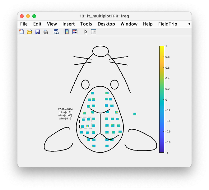
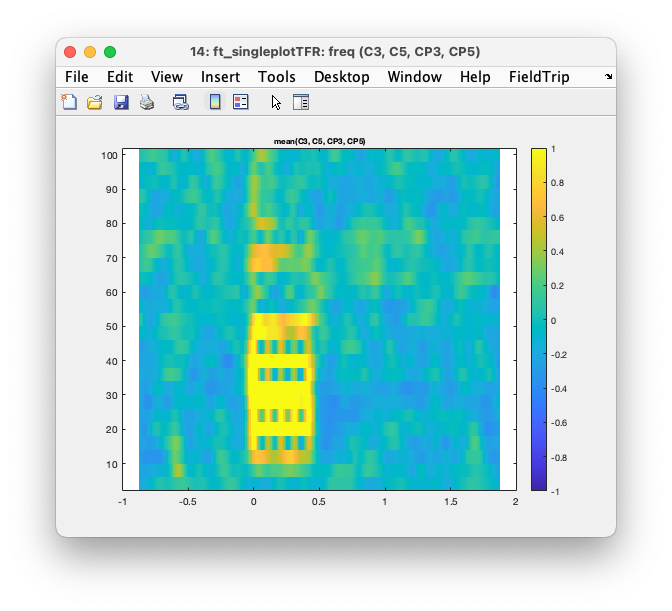
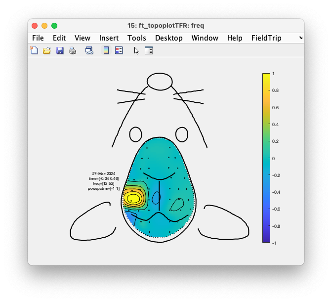
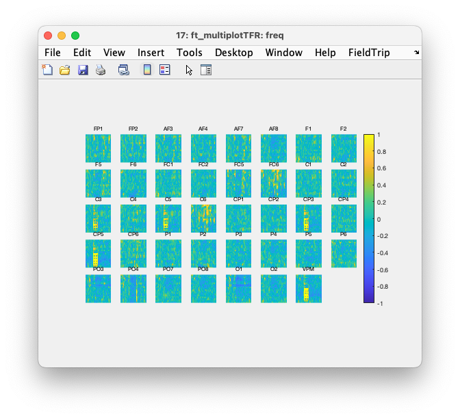
The results of the time-frequency analysis can be plotted with ft_multiplotTFR and ft_singleplotTFR. To visualize the power changes due to stimulation and to compare the power over frequencies, we perform a normalization with respect to the baseline. By specifying cfg.baselinetype = 'relchange' we compute the relative change, which is the power minus the average power in the baseline, divided the average power in the baseline.
% visualization of all EEG channels
cfg                   = [] ;
cfg.xlim              = [-1 2];
cfg.ylim              = [4 100];
cfg.zlim              = [-1.0 1.0];
cfg.colorbar          = 'yes';
cfg.layout            = 'layout42.mat'; % from disk
cfg.showoutline       = 'yes';
cfg.baseline          = [-0.5 0];
cfg.baselinetype      = 'relchange' ;
ft_multiplotTFR(cfg, freq);
Figure: Interactive plot of all channels using ft_multiplotTFR.
Again with cfg.interactive = 'yes', which is the default, you can select one or multiple channels, click on them and get an average TFR over those channels,. In that average you can make a time and frequency selection, click in it, and get a spatial topopgraphy of the relative power over all channels in that time-frequency range.
Figure: Interaction results in a ft_singleplotTFR figure.
Figure: Interaction results in a ft_topoplotTFR figure.
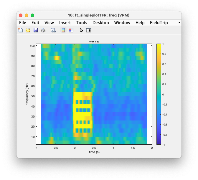
You can also explicitly plot the TFR for a specific channel. Here we use it for the VMP channel as that channel is not contained in the 2D layout of the EEG array and hence not plotted with ft_multiplotTFR when we specify cfg.layout = 'layout42.mat'.
% single channel visualization
cfg                   = [] ;
cfg.channel           = 'VMP'; % you can also specify multiple, it will then average
cfg.xlim              = [-1 2];
cfg.ylim              = [4 100];
cfg.zlim              = [-1.0 1.0];
cfg.colorbar          = 'yes';
cfg.baseline          = [-0.2 0];
cfg.baselinetype      = 'relchange' ;
ft_singleplotTFR(cfg, freq);
xlabel('time (s)')
ylabel('frequency (Hz)')
Figure: Plot of VMP with ft_singleplotTFR.
You can also visualize the TFRs sequentially over all channels. An advantage compared to the previous ft_multiplotTFR figure is that channel VMP is now also plotted. A disadvantage is that we cannot make a meaningful topography out of this.
% visualization of all EEG channels, not topographically arranged
cfg                   = [] ;
cfg.xlim              = [-1 2];
cfg.ylim              = [4 100];
cfg.zlim              = [-1.0 1.0];
cfg.colorbar          = 'yes';
cfg.layout            = 'ordered'; % see FT_PREPARE_LAYOUT
cfg.showlabels        = 'yes';
cfg.baseline          = [-0.5 0];
cfg.baselinetype      = 'relchange' ;
ft_multiplotTFR(cfg, freq);
Figure: Plot of all channels, not using layout but ordered.
Anatomical processing and construction of the volume conduction model
Reading and coregistring the anatomical data
The anatomical MRI is originally obtained from http://brainatlas.mbi.ufl.edu, but is also available from our download server.
mri = ft_read_mri('Num1_MinDef_M_Normal_age12_num10.hdr')

figure
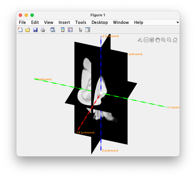
ft_determine_coordsys(mri, 'interactive', 'no')
Figure: determine the initial units and coordinate system.
This gives a figure that shows the origin as a white sphere, the x-axis in red, the y-axis in green and the z-axis in blue (remember “RGB”). The positive x-axis points to right, the y-axis to inferior, the z-axis to anterior. Hence the MRI is expressed in a RIA (right-inferior-anterior) coordinate system.
We notice that the origin is not at Bregma, nor at the interaural point. Both the direction of the axes and the origin are inconsistent with the desired coordinate system, hence we have to realign the anatomical MRI.
Furthermore, we notice that the unit has been estimated as ‘cm’ and that the scale of the mouse brain is incorrect. The white sphere is 1 cm in diameter, so the brain is way too large. We can correct and check this, now plotting it with 15 mm axes and a 1 mm white sphere at the origin.
% fix the initial coordinate system and units
mri.coordsys = 'ria'
mri.unit = 'mm'

% plot once more
figure
ft_determine_coordsys(mri, 'interactive', 'no', 'axisscale', 0.1)
… using the graphical user-interface
We can use the ft_volumerealign function to coregister the anatomical MRI to the desired coordinate system. There are multiple coordinate systems in which the anatomy of the brain and head can be described, but here we want to use the Paxinos-Franklin coordinate system which uses Bregma and Lambda as anatomical landmarks (or fiducials).
cfg = [];
cfg.coordsys  = 'paxinos';
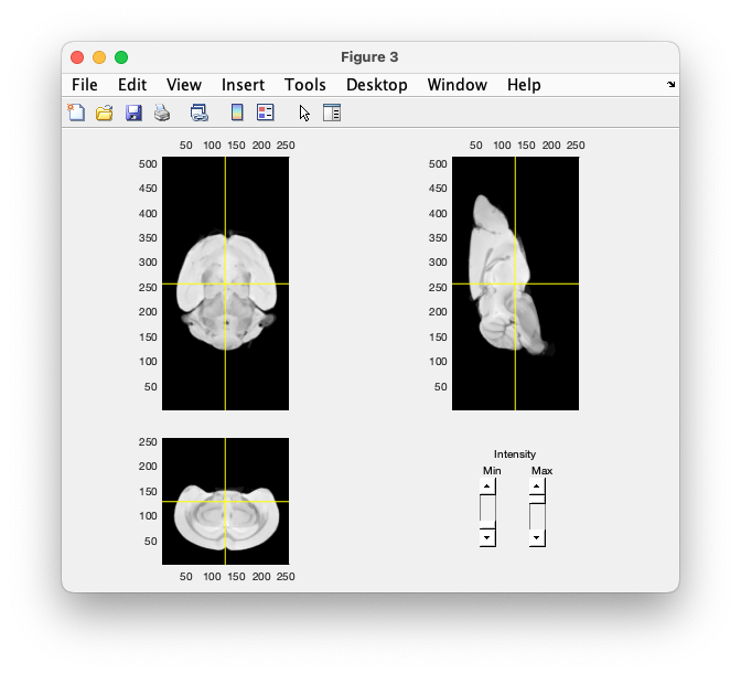
mri_realigned = ft_volumerealign(cfg, mri);
Figure: interactively align to the Paxinos coordinate system using ft_volumerealign.
The anatomical MRI is displayed in three orthogonal plots. You have to visually identify the anatomical landmark location and press “b” for bregma, “l” for lambda and “z” for a midsagittal point. Using “f” you can toggle the landmarks or fiducials on and off. Once you are happy with their placement, you press “q” and the realigned mri is returned:
mri_realigned =
          anatomy: [256x256x512 double]
              dim: [256 256 512]
              hdr: [1x1 struct]
        transform: [4x4 double]
    transformorig: [4x4 double]
             unit: 'mm'
         coordsys: 'paxinos'
              cfg: [1x1 struct]
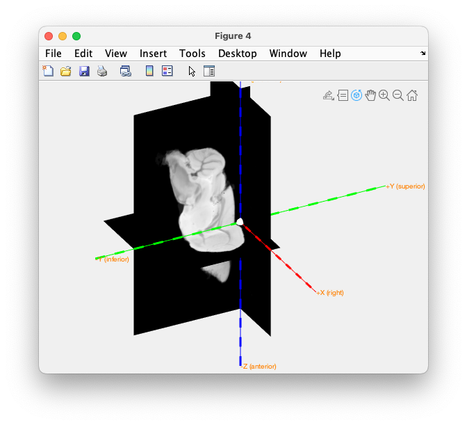
We can check the coordinate axes once more. Besides printing the axis labels for X, Y and Z, it now also shows the interpretation of the directions as “right”, “superior”, “posterior”.
figure
ft_determine_coordsys(mri_realigned, 'interactive', 'no', 'axisscale', 0.1)
Figure: check the Paxinos coordinate system.
… by specifying landmarks
We can also explicitly determine the location of three landmarks (expressed in the original coordinate system) using ft_sourceplot and write them down.
cfg = [];
ft_sourceplot(cfg, mri)
By clicking in the figure, we establish that the landmarks (in mm) are:
% FIXME these numbers seem to be incorrect
bregma      = [0 -5.0 2.5];
lambda      = [0 -5.0 2.0];
midsagittal = [0.2 -0.7 -2.0];
The ft_headcoordinates function provides the homogenous transformation matrix to rotate and translate the MRI into the Paxinos coordinate system.
head2paxinos = ft_headcoordinates(bregma, lambda, midsagittal, 'paxinos')

head2paxinos =
    0.9994    0.0225    0.0256   -0.0009
    0.0225   -0.9997    0.0006   -4.4011
    0.0256   -0.0000   -0.9997    3.8987
         0         0         0    1.0000
We can apply this homogenous transformation matrix to the MRI with
vox2head    = mri.transform;
vox2paxinos = head2paxinos * vox2head;

mri_realigned           = mri;         % copy the original MRI
mri_realigned.transform = vox2paxinos; % update the homogenous transformation matrix
mri_realigned.coordsys = 'paxinos';
It is useful to also explicitly specify the coordinate system in the anatomical MRI. It is used by ft_sourceplot and various other functions to check whether various geometrical objects are expressed in the same coordinate system.
Reslicing the anatomical MRI
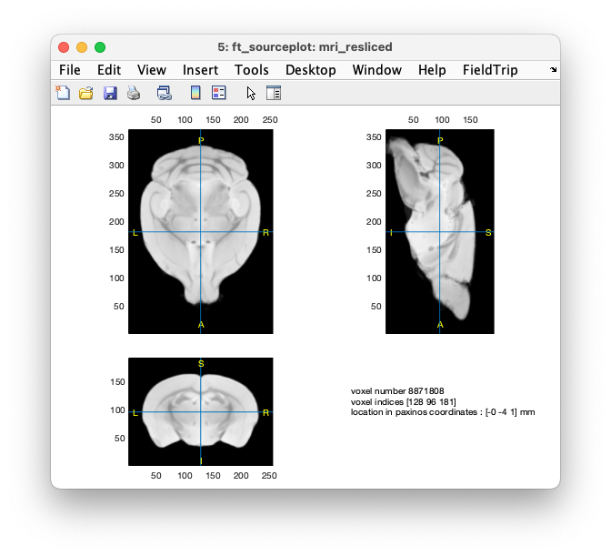
After coregistration of the MRI with the Paxinos coordinate system, it is convenient to reslice it, i.e., to interpolate the greyscale values on a 3-D grid that is nicely aligned with the cardinal axes.
cfg = [];
cfg.xrange = [-6 6];
cfg.yrange = [-8 1];
cfg.zrange = [-7 10];
cfg.resolution = 0.0470;
mri_resliced = ft_volumereslice(cfg, mri_realigned)

figure
ft_sourceplot(cfg, mri_resliced)
Figure: anatomical MRI after realigning and reslicing
Reading and coregistring the anatomical atlas
On http://brainatlas.mbi.ufl.edu (and our download server) there is also an anatomically labeled version of the same brain available. We can use this as anatomical atlas.
atlas = ft_read_mri('Num1_MinDef_M_Normal_age12_num10Atlas.hdr')
Since the original anatomical and labeled MRI are expressed in the same coordinate system, we can apply the same transformation to the atlas. Again, we also fix the units and specify the coordinate system.
atlas_realigned             = atlas;
atlas_realigned.transform   = mri_realigned.transform;
atlas_realigned.unit        = mri_realigned.unit;
atlas_realigned.coordsys    = mri_realigned.coordsys;
We can visualise the atlas in the same way as the anatomical MRI.
cfg = [];
ft_sourceplot(cfg, atlas);
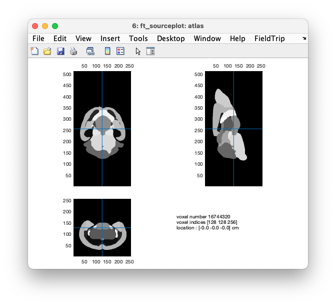
Figure: plotting the atlas as an anatomical MRI, notice that all values are integers
You can see (by clicking around) that it contains integer values. Each area with the same integer value is a single region.
The Analyze (hdr+img) files that contain the atlas do not include the labels of the different tissue types. We can fix this and manually assign the labels from this paper.
  % rename "anatomy" into "tissue"
  atlas_realigned.tissue = atlas_realigned.anatomy;
  atlas_realigned = rmfield(atlas_realigned, 'anatomy');

  % add a "tissuelabel" cell-array with the names
  atlas_realigned.tissuelabel = {'Hippocampus', 'External_capsule', 'Caudate_putamen', ...
    'Ant_commissure', 'Globus_pallidus', 'Internal_Capsule', 'Thalamus', ...
    'Cerebellum', 'Superior_colliculi', 'Ventricles', 'Hypothalamus', ...
    'Inferior_colliculi', 'Central_grey', 'Neocortex', 'Amygdala', ...
    'Olfactoryt_bulb', 'Brain_stem', 'Rest_of_Midbrain', ...
    'BasalForebrain_septum', 'Fimbria'};
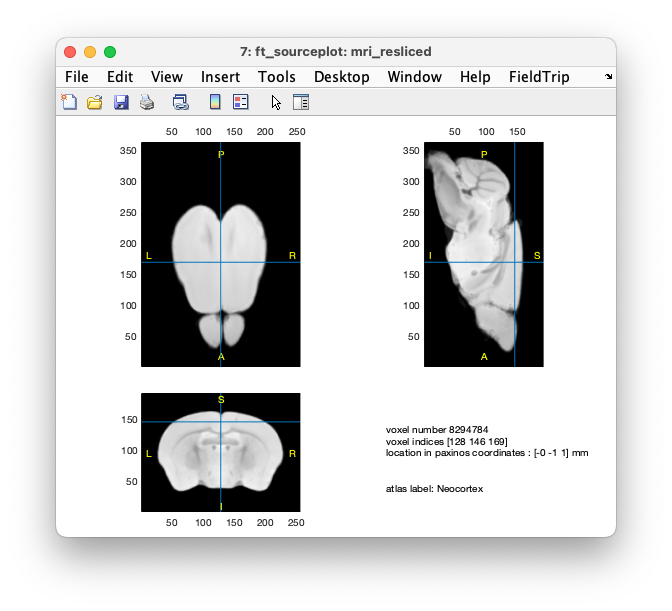
With the correct labels, we can use ft_sourceplot to plot the anatomical MRI and show the corresponding atlas label by clicking on a location in the brain.
cfg = [];
cfg.atlas = atlas_realigned;
ft_sourceplot(cfg, mri_resliced)
Figure: resliced anatomical MRI, with the anatomical labels from the realigned atlas
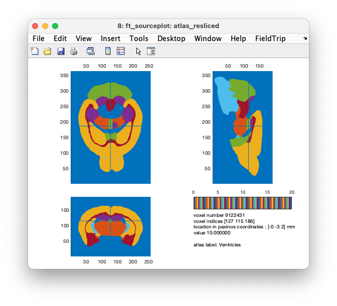
It is also possible to explore only the atlas itself, using the anatomical labels in the atlas. For that it is again convenient to reslice the atlas so that the voxels are aligned with the canonical axes. Note that we do not want to interpolate the values, since a voxel that happens to be in between tissue 1 and 2 cannot be assumed to correspond to tissue label 2.
cfg = [];
cfg.xrange = [-6 6];
cfg.yrange = [-8 1];
cfg.zrange = [-7 10];
cfg.resolution = 0.0470;
cfg.method = 'nearest'; % take the nearest value, do not interpolate
atlas_resliced = ft_volumereslice(cfg, atlas_realigned)

cfg = [];
cfg.atlas = atlas_resliced;
cfg.funparameter = 'tissue';
cfg.funcolormap = 'lines';
ft_sourceplot(cfg, atlas_resliced)
Figure: realigned and resliced anatomical atlas, including labels
Construction of the forward model
Source reconstruction requires a forward model that allows us to compute the relation between the activity for each model dipole and the potential distribution at the electrodes. The forward model is based on a geometrical model for the head, the conductive properties of the tissues, and the electrode positions. Furthermore, the sourcemodel specifies the locations at which we want to probe for the activity. If we have the headmodel, the sourcemodel and electrodes, we can compute the so-called leadfield matrices which are used for the source reconstruction.
Make segmentation of the brain and skull
We start with a histogram of the grey-scale values
hist(mri_resliced.anatomy(:), 100)
axis(1.0e+06 * [-0.001    0.017   -0.010    1.00]); % ugh!
From the histogram we can determine a threshold in between the two bumps and use that to make a binary image of the brain.
% start with a copy
mri_resliced_segmented = mri_resliced;

mri_resliced_segmented.brain = mri_resliced.anatomy>6000;

se = strel('sphere', 9); % see "doc strel"
mri_resliced_segmented.skull = imdilate(mri_resliced.brain, se);

combined = mri_resliced_segmented.skull + mri_resliced_segmented.brain;

figure
for i=1:15
  subplot(5, 3, i)
  imagesc(squeeze(combined(:,(i+1)*10,:)))
  axis equal; axis tight; axis off
end
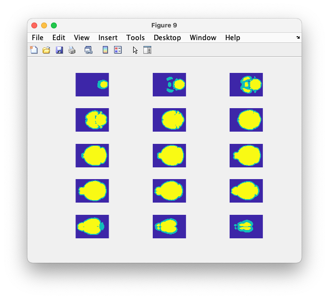
The skull shows up with integer value 1 and the brain (which is fully enclosed in the skull) shows up with integer value 2.
Figure: segmented brain in yellow, dilated to approximate the skull in green
Make mesh of the brain-skull and skull-skin boundary
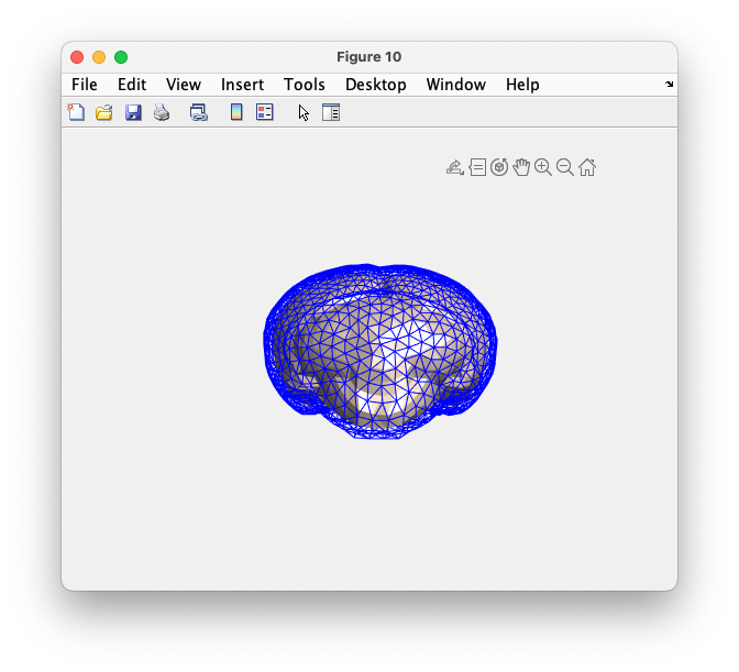
In the previous section we performed a segmentation to extract the brain and skull. Since we use an in-vitro MRI without skull, a virtual skull was made from the brain surface by image dilation. To construct the surfaces of the boundaries, we use the ft_prepare_mesh to get the triangulated meshes for skull and brain.
cfg             = [];
cfg.tissue      = {'skull', 'brain'};  % value 1 is skull, value 2 is brain
cfg.numvertices = [1500, 1500];
mesh            = ft_prepare_mesh(cfg, mri_resliced_segmented);

figure
ft_plot_mesh(mesh(1), 'facecolor', 'none', 'edgecolor', 'b')
ft_plot_mesh(mesh(2), 'facecolor', 'skin', 'edgecolor', 'none')
camlight
Figure: triangulated mesh for the brain and skull surface
Make BEM volume conduction model
After making up volume objects, we perform the ft_prepare_headmodel for assigning the electrical property of volumes. From the literature in human study, the brain conductivity ranges from 0.12-0.48/Ω.m [ref 1-3], and the human skull from 0.006-0.015/Ω.m [ref 4,5] or even higher as 0.032-0.080/Ω.m [ref 5]. According to another studies for the conductivity ratio between skull and brain, they reported numerical value with large variation the ranges from 25 to 80 times [ref 6]. It is hard to specify the brain-to-skull conductivity ratio from these values with such large variations. In this step, we just assign conductivities applying to 80 times ratio between skull and brain.
- Nicholson, Paul W. “Specific impedance of cerebral white matter.” Experimental neurology 13.4 (1965): 386-401.
- Gonçalves, Sónia I., et al. “In vivo measurement of the brain and skull resistivities using an EIT-based method and realistic models for the head.” Biomedical Engineering, IEEE Transactions on 50.6 (2003): 754-767.
- Oostendorp, Thom F., Jean Delbeke, and Dick F. Stegeman. “The conductivity of the human skull: results of in vivo and in vitro measurements.” Biomedical Engineering, IEEE Transactions on 47.11 (2000): 1487-1492.
- Hoekema, R., et al. “Measurement of the conductivity of skull, temporarily removed during epilepsy surgery.” Brain topography 16.1 (2003): 29-38.
- Rush, S., and Daniel A. D. “Current distribution in the brain from surface electrodes.” Anesthesia & Analgesia 47.6 (1968): 717-723.
- Lai, Y., et al. “Estimation of in vivo human brain-to-skull conductivity ratio from simultaneous extra-and intra-cranial electrical potential recordings.” Clinical neurophysiology 116.2 (2005): 456-465.
OpenMEEG is an external package that solves the forward problem. It implements a Boundary Element Method (BEM) and provides accurate solutions when dealing with realistic head models. As we mentioned above in the segmentation section, we are computing the BEM for two layers (brain and skull).
cfg = [];
cfg.tissue = {'skull', 'brain'};
cfg.conductivity = [0.33/80, 0.33];
cfg.method = 'openmeeg';
headmodel = ft_prepare_headmodel(cfg, mesh);

headmodel =
             bnd: [1x2 struct]
            cond: [0.0041 0.3300]
    skin_surface: 1
          source: 2
             mat: [5996x5996 double]
            type: 'openmeeg'
            unit: 'mm'
             cfg: [1x1 struct]
Specification of 3D electrode positions
We need to specify the 3D electrode positions relative to the BEM model of the head. The electrode positions are expressed relative to the middle of the 4th row, as that was aligned with the bregma point as the origin.
loc = [
  -1.461   3.457  0.437357631 % 1st row, Fp2
   1.461   3.457  0.437357631
  -1.461   2.396  0.328018223 % 2nd row
   1.461   2.396  0.328018223
  -2.147   2.396  0.482915718
   2.147   2.396  0.482915718
  -1.461   1.131  0.236902050 % 3rd row
   1.461   1.131  0.236902050
  -2.396   1.131  0.501138952
   2.396   1.131  0.501138952
  -1.710   0      0.264236902 % 4th row
   1.710   0      0.264236902
  -3.243   0      0.738041002
   3.243   0      0.738041002
  -1.559  -0.989  0.118451025 % 5th row
   1.559  -0.989  0.118451025
  -2.512  -0.989  0.291571754
   2.512  -0.989  0.291571754
  -3.510  -0.989  0.765375854
   3.510  -0.989  0.765375854
  -1.666  -2.254  0.027334852 % 6th row
   1.666  -2.254  0.027334852
  -2.673  -2.254  0.118451025
   2.673  -2.254  0.118451025
  -3.670  -2.254  0.610478360
   3.670  -2.254  0.610478360
  -1.684  -3.332  0.018223235 % 7th row
   1.684  -3.332  0.018223235
  -2.949  -3.332  0.346241458
   2.949  -3.332  0.346241458
  -4.009  -3.332  0.847380410
   4.009  -3.332  0.847380410
  -1.675  -4.695  0.291571754 % 8th row
   1.675  -4.695  0.291571754
  -2.619  -4.695  0.464692483
   2.619  -4.695  0.464692483
  -1.764  -5.702  0.473804100 % 9th row, O2
   1.764  -5.702  0.473804100
];
To confirm the alignment between the headmodel and electrode positions, we make a 3D figure using the following code.
figure
ft_plot_mesh(mesh(1), 'facecolor', 'skin', 'edgecolor', 'b');
hold on
alpha 0.9 % slightly transparent
camlight
plot3(loc(:, 1), loc(:, 2), loc(:, 3), '*k');
hold off
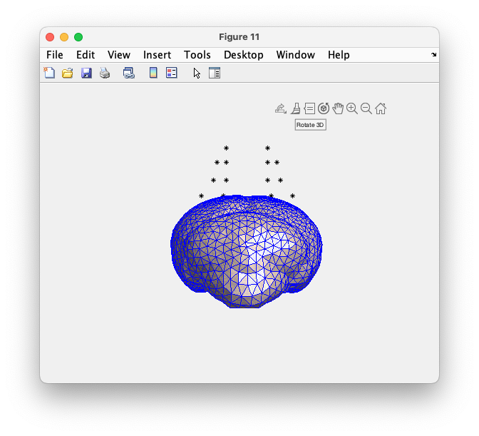
Figure: triangulated mesh of the skull with the electrodes, clearly not aligned
You see that this is not what you would expect, as the electrode positions are totally not aligned with the skull surface. This is because they are not expressed in the correct coordinates. We can fix this by using the known location of the anatomical landmarks. We again use the ft_headcoordinates function with the input variables bregma, lambda, and midsagittal.
- The bregma point should be at at [0, 0, 0].
- The lambda point should be at [0, y, 0] aligned with the anterio-parietal axis.
- The midsagittal point should be at a location inside the brain compared to the electrode array, so a little bit down.
The bregma and lambda points can be found by averaging the electrode positions on their left and right.
bregma      = mean(loc(11:12, :));      % in between FC2 and FC1
lambda      = mean(loc([27 28], :));    % in between P2 and P1
midsagittal = bregma + [0 0 1];         % in the positive z direction

elec2paxinos = ft_headcoordinates(bregma, lambda, midsagittal, 'paxinos');
Subsequently, we can apply the transformation matrix to the electrode position. We first organize the electrode positions in a MATLAB structure, in line with the FieldTrip description of electrodes.
elec = [];
elec.elecpos  = loc;
elec.unit     = 'mm';
elec.label    = {
  'FP2';'FP1';
  'AF4';'AF3';'AF8';'AF7';...
  'F2';'F1';'F6';'F5';
  'FC2';'FC1';'FC6';'FC5';...
  'C2';'C1';'C4';'C3';'C6';'C5';
  'CP2';'CP1';'CP4';'CP3';'CP6';'CP5';...
  'P2';'P1';'P4';'P3';'P6';'P5';
  'PO4';'PO3';'PO8';'PO7';
  'O2';'O1'
};

% apply the transformation
elec_realigned = ft_transform_geometry(elec2paxinos, elec);

% remember the coordinate system that we assigned
elec_realigned.coordsys = 'paxinos';
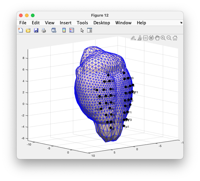
We check the result of co-registration between the headmodel and electrodes in a 3D figure.
figure
ft_plot_mesh(mesh(1), 'facecolor', 'skin', 'edgecolor', 'b');
hold on
ft_plot_sens(elec_realigned, 'elecsize', 20, 'label', 'label');
hold off
axis on
grid
alpha 0.8
camlight
material dull
view(-220, 10)
Figure: triangulated mesh of the skull with the aligned electrodes
After the co-registration there are still some small gaps between the electrode positions and the skull surface. That is not something to worry about: when computing the BEM solutions, FieldTrip will automatically project the 3D electrode positions orthogonally onto the outermost surface. However, we can also do an explicit projection of the electrodes on the surface.
cfg = [];
cfg.method = 'project';
cfg.headshape = mesh(1);
elec_projected = ft_electroderealign(cfg, elec_realigned);
Deal with differences in animal size
As we discussed before, in these mouse EEG recordings the electrode grid does not scale along with the size of the animal. Consequently, the position of the electrodes relative to the brain depends on the head size. This affects the topographic plotting of channel level data, the comparison (group stats) of channel-level data from multiple animals, and the electrode positions and volume conduction model used for source reconstruction.
The principled solution is that the experimentally measured lambda-bregma distance (or some other measure of head size) is used to scale the background image that is used in the channel layout for plotting. We could apply the same scaling to the volume conduction model of the head.
The more pragmatic solution that we use here is to inverse-scale the electrodes and keep the head size constant. Effectively the result is the same, but it is easier to manage as it makes the source-level results directly comparable over animals. This is comparable to using an MNI template MRI and headmodel for human EEG source reconstruction.
For this specific animal no further scaling is needed.
Make sourcemodel and leadfields
With ft_prepare_sourcemodel we construct a regular grid of dipoles that spans the complete brain.
cfg            = [];
cfg.elec       = elec_projected;
cfg.headmodel  = headmodel;
cfg.xgrid      = -6:0.25:6;
cfg.ygrid      = -8:0.25:1;
cfg.zgrid      = -7:0.25:10;
cfg.unit       = 'mm';
sourcemodel    = ft_prepare_sourcemodel(cfg);
With ft_prepare_leadfield we can compute the leadfield matrices that specify the spatial topography on all EEG electrodes for each of the dipoles in the source model.
cfg                 = [];
cfg.sourcemodel     = sourcemodel;
cfg.elec            = elec_projected;
cfg.headmodel       = headmodel;
cfg.reducerank      = 3;
cfg.normalize       = 'yes';
cfg.channel         = elec_projected.label;
leadfield           = ft_prepare_leadfield(cfg);

leadfield =
        xgrid: [1x40 double]
        ygrid: [1x29 double]
        zgrid: [1x59 double]
          dim: [40 29 59]
          pos: [68440x3 double]
    leadfield: {68440x1 cell}
       inside: [68440x1 logical]
         unit: 'mm'
          cfg: [1x1 struct]
Source reconstruction
The beamforming technique that we also use for EEG and MEG source reconstruction is based on a spatial filter. The DICS spatial filter is derived from the cross-spectral density matrix, which is the frequency-domain counterpart of the covariance matrix.
Calculating the cross spectral density matrix
Before computing the cross-spectral density matrix, we make a subselection of the data in the pre-stimulus and in the post-stimulus interval. We will use these later to make a contrast between the two conditions.
% make selections in the data
cfg          = [];
cfg.toilim   = [-0.5500 -0.0505]; % aim for exactly 1000 samples
dataPre      = ft_redefinetrial(cfg, data_reref);

cfg          = [];
cfg.toilim   = [-0.0500 0.4495]; % aim for exactly 1000 samples
dataPost     = ft_redefinetrial(cfg, data_reref);
The cross-spectrum is computed from the Fourier transformed data and returned as output by ft_freqanalysis when we specify cfg.output = 'powandcsd'. The frequency of interest is 10 Hz and we use multitapering with a smoothing window of +/-4 Hz:
% compute the cross-spectral density
cfg           = [];
cfg.method    = 'mtmfft';
cfg.output    = 'powandcsd';
cfg.tapsmofrq = 4;
cfg.foilim    = [10 10];
freqPre       = ft_freqanalysis(cfg, dataPre);

cfg           = [];
cfg.method    = 'mtmfft';
cfg.output    = 'powandcsd';
cfg.tapsmofrq = 4;
cfg.foilim    = [10 10];
freqPost      = ft_freqanalysis(cfg, dataPost);
To check the selected data and computations so far, we can compute and plot the difference between the power spectrum in the Post and Pre time windows as dB change using ft_math. Note that for frequency data without time axis (as here) you should not use ft_topoplotTFR for plotting, but ft_topoplotER (and idem for multiplot and singleplot).
cfg           = [];
cfg.parameter = 'powspctrm';
cfg.operation = '10*log10(x1/x2)'; % convert to dB difference
freqContrast  = ft_math(cfg, freqPost, freqPre);

cfg             = [];
cfg.layout      = 'layout42.mat'; % from disk
cfg.zlim        = 'maxabs';
cfg.showoutline = 'yes';
cfg.marker      = 'labels';
cfg.colorbar    = 'yes';
ft_topoplotER(cfg, freqContrast);
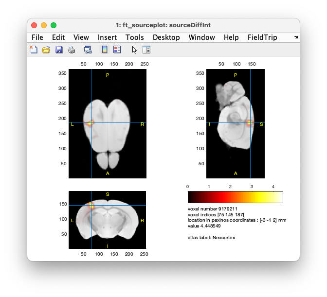
Using the covariance matrices and the leadfield matrices, a spatial filtering is calculated and estimated the dipole intensity for each grid point. By applying the filter to the Fourier transformed data we can then estimate the power for neural activity by optogenetic stimuli (10 Hz). This results in a power estimate for each grid point. To get normalized index for the neural activity we have to do the spatial filtering both pre-stimulus and post-stimulus.
cfg                   = [];
cfg.elec              = elec_projected;
cfg.channel           = elec_projected.label;
cfg.method            = 'dics';
cfg.frequency         = 10;
cfg.sourcemodel       = leadfield;
cfg.headmodel         = headmodel;
cfg.dics.projectnoise = 'yes';
cfg.dics.kappa        = 37;  % the rank of the EEG data
cfg.dics.lambda       = '5%';
cfg.dics.keepfilter   = 'no';
cfg.dics.realfilter   = 'yes';
sourcePre             = ft_sourceanalysis(cfg, freqPre);
sourcePost            = ft_sourceanalysis(cfg, freqPost);

% the units are not stored, and when guessed later on will be incorrect
% copy the 'mm' over from the leadfield and sourcemodel structures
sourcePre.unit  = leadfield.unit;
sourcePost.unit = leadfield.unit;
To calculate neural activity index is the same like below equation. The function ft_sourceinterpolate interpolates the source reconstructed activity or a statistical distribution onto the voxels or vertices of an anatomical description of the brain (MRI with atlas).
cfg = [];
cfg.parameter = 'pow';
cfg.operation = '10*log10(x1/x2)'; % convert to dB difference
sourceDiff = ft_math(cfg, sourcePost, sourcePre);

% copy the 'mm' over from the leadfield and sourcemodel structures
sourceDiff.unit = leadfield.unit;

cfg                 = [];
cfg.parameter       = 'pow';
sourceDiffInt       = ft_sourceinterpolate(cfg, sourceDiff , mri_resliced);
Visualize the source reconstruction
cfg               = [];
cfg.atlas         = atlas_resliced;
cfg.method        = 'ortho'; % you can also use 'slice'
cfg.funparameter  = 'pow'; % for color
cfg.maskparameter = 'pow'; % for opacity
cfg.funcolorlim   = 'zeromax';
cfg.opacitylim    = 'zeromax';
ft_sourceplot(cfg, sourceDiffInt);
Figure: source reconstruction, contrast of the activity versus baseline
Suggested further reading
- Video that describes the high-density mouse EEG array: http://www.jove.com/video/2562/high-density-eeg-recordings-freely-moving-mice-using-polyimide-based
- PLoS ONE (2013) paper about the mouse EEG source reconstruction: http://www.ncbi.nlm.nih.gov/pubmed/24244506
- Comparable monkey ECoG: http://www.ncbi.nlm.nih.gov/pubmed/19436080
- Comparable rat ECoG part 1: http://www.ncbi.nlm.nih.gov/pubmed/24820913
- Comparable rat ECoG part 2: http://www.ncbi.nlm.nih.gov/pubmed/24814253
