Computation of virtual MEG channels in source-space
In the extended beamformer tutorial we identified two potentially interesting regions, one which produces visual gamma-band activity and the other which is coherent with the EMG sensors. If you want to continue analyzing those two regions it is pretty unhandy to juggle around with the two source structures all the time. Also, using the DICS method you do not get a time-resolved signal of these sources. In the following example we will show how you can create virtual channels out of these two sources, which can then be used for further analysis, for example connectivity analysis.
Compute the spatial filter for the region of interest
After having done all steps in the extended beamformer tutorial, you have the preprocessed data, two source structures, and a headmodel. You can also get these from the download server:
We will now determine the positions on which the cortico-muscular coherence is the largest and the position where the induced visual gamma activity is largest:
[maxval, maxcohindx] = max(source_coh_lft.avg.coh);
source_coh_lft.pos(maxcohindx, :)

ans =
      3.2000   -0.6000   7.4000

[maxval, maxpowindx] = max(source_diff.avg.pow);
source_diff.pos(maxpowindx, :)

ans =
      0.4000   -8.8000    2.6000
The cortical position is expressed in MNI space according to the template brain we used for warping and in centimeter. Relative to the anterior commissure (AC) the coherence peak position is 3.2 cm towards the right side of the brain, -0.6 towards the front of the AC (i.e., 0.6 cm towards the back!) and 7.4 cm towards the vertex. The visual gamma peak is 0.4 cm towards the right of the brain , -8.8 cm to the front of the AC (i.e. 8.6 cm to the back) and 2.6 cm to the top.
The ft_sourceanalysis methods are usually applied to the whole brain using a regular 3-D grid or using a triangulated cortical sheet. You can also just specify the location of a single or multiple points of interest with cfg.sourcemodel.pos and the LCMV beamformer will simply be performed at the location of interest. Note that we have to use subject-specific coordinates here and not the MNI template.
The LCMV beamformer spatial filter for the location of interest will pass the activity at that location with unit-gain, while optimally suppressing all other noise and other source contributions to the MEG data. The LCMV implementation in FieldTrip requires the data covariance matrix to be computed with ft_timelockanalysis.
cfg                   = [];
cfg.covariance        = 'yes';
cfg.channel           = 'MEG';
cfg.vartrllength      = 2;
cfg.covariancewindow  = 'all';
tlock = ft_timelockanalysis(cfg, data_cmb);

cfg                     = [];
cfg.method              = 'lcmv';
cfg.headmodel           = hdm;
cfg.sourcemodel.pos     = sourcemodel.pos([maxcohindx maxpowindx], :);
cfg.sourcemodel.inside  = true(2,1);
cfg.unit                = sourcemodel.unit;
cfg.lcmv.keepfilter     = 'yes';
source_idx = ft_sourceanalysis(cfg, tlock);
The source reconstruction contains the estimated power and the source-level time series of the averaged ERF, but here we are not interested in those. The cfg.keepfilter option results in the spatial filter being kept in the output source structure. That spatial filter can be used to reconstruct the single-trial time series as a virtual channel by multiplying it with the original MEG data.
Extract the virtual channel time series
beamformer_lft_coh = source_idx.avg.filter{1};
beamformer_gam_pow = source_idx.avg.filter{2};

chansel  = ft_channelselection('MEG', data_cmb.label); % find MEG sensor names
chanindx = match_str(data_cmb.label, chansel);         % find MEG sensor indices

coh_lft_data = [];
coh_lft_data.label = {'coh_lft_x', 'coh_lft_y', 'coh_lft_z'};
coh_lft_data.time = data_cmb.time;

gam_pow_data = [];
gam_pow_data.label = {'gam_pow_x', 'gam_pow_y', 'gam_pow_z'};
gam_pow_data.time  = data_cmb.time;

for i=1:length(data_cmb.trial)
  coh_lft_data.trial{i} = beamformer_lft_coh * data_cmb.trial{i}(chanindx,:);
  gam_pow_data.trial{i} = beamformer_gam_pow * data_cmb.trial{i}(chanindx,:);
end
The LCMV spatial filter is computed here without applying any time-domain filters. Consequently, it will have to suppress all noise in the data in all frequency bands. The spatial filter derived from the broadband data allows us to compute a broadband source level time series.
If you would know that the subsequent analysis would be limited to a specific frequency range in the data (e.g., everything above 30 Hz), you could first apply a filter using ft_preprocessing (e.g., cfg.hpfilter=yes and cfg.hpfreq=30) prior to computing the covariance and the spatial filter.
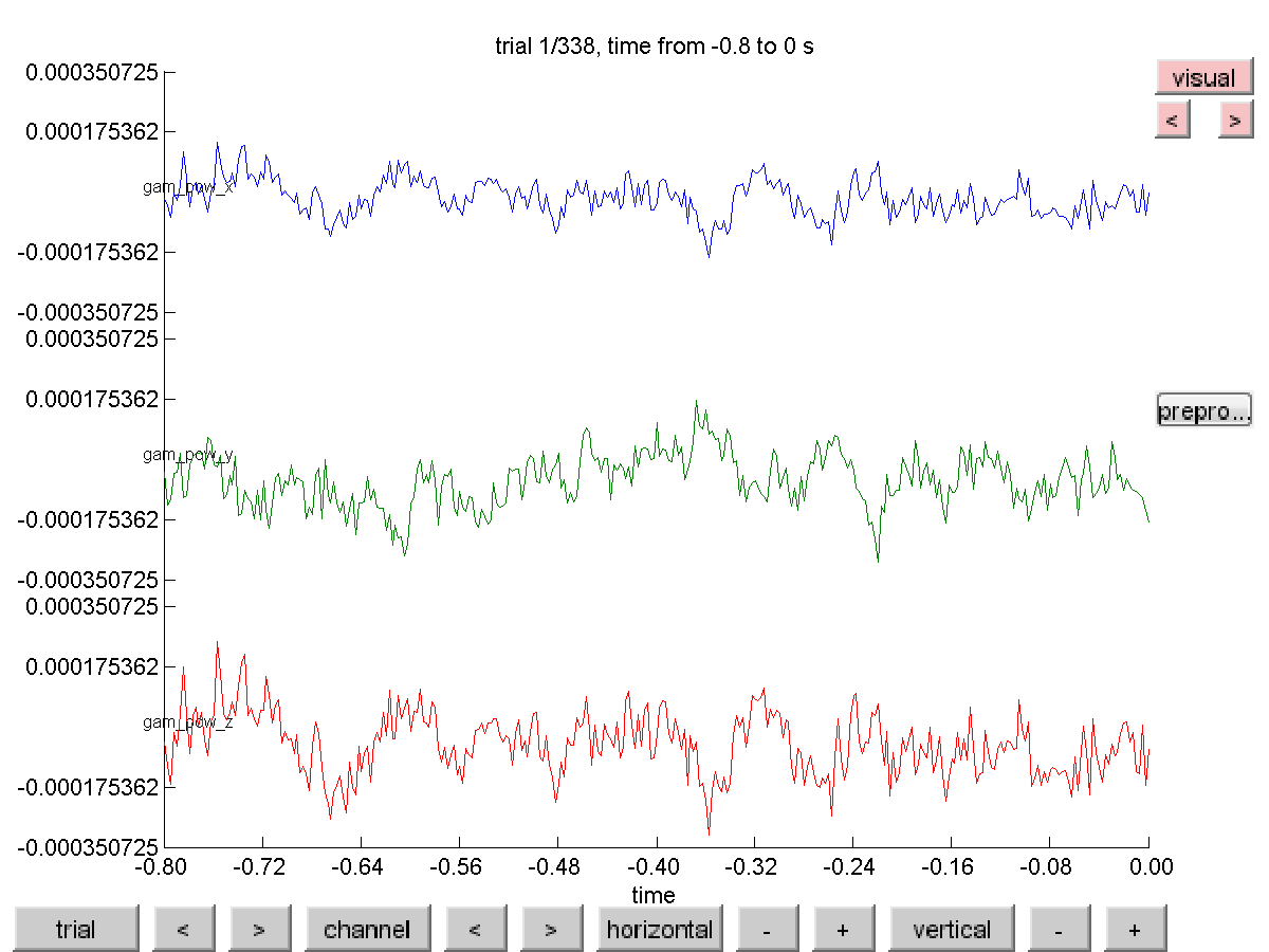
The structures coh_lft_data and gam_pow_data resemble the raw-data output of ft_preprocessing and consequently can be used in any follow-up function. You can for example visualize the single-trial virtual channel time series using ft_databrowser.
cfg = [];
cfg.viewmode = 'vertical';  % you can also specify 'butterfly'
ft_databrowser(cfg, gam_pow_data);
Notice that the reconstruction contains three channels, for the x-, the y- and the z-component of the equivalent current dipole source at the location of interest.
