Simulating and estimating, what about model (mis)match?

Introduction

Background

The brain is organized in functional units, which at the smallest level consists of neurons, and at higher levels consists of larger neuronal populations. Functional localization studies consider the brain to be organized in specialized neuronal modules corresponding to specific areas in the brain. These functionally specialized brain areas (e.g., visual cortex area V1, V2, V4, MT, …) have to pass information back and forth along anatomical connections. Identifying these functional connections and determining their functional relevance is the goal of connectivity analysis and can be done using ft_connectivityanalysis and associated functions.

The nomenclature for connectivity analysis can be adopted from graph theory, in which brain areas correspond to nodes or vertices and the connections between the nodes is given by edges. One of the fundamental challenges in the analysis of brain networks from MEG and EEG data lies not only in identifying the “edges”, i.e. the functional connections, but also the “nodes”. The remainder of this tutorial will only explain the methods to characterize the edges, but will not go into details for identifying the nodes. The beamformer tutorial and corticomuscular coherence tutorial provide more pointers to localizing the nodes.

Many measures of connectivity exist, and they can be broadly divided into measures of functional connectivity (denoting statistical dependencies between measured signals, without information about causality/directionality), and measures of effective connectivity, which describe directional interactions. If you are not yet familiar with the range of connectivity measures (i.e., mutual information, coherence, granger causality), you may want to read through some of the papers listed under the method references for connectivity analysis

After the identification of the network nodes and the characterization of the edges between the nodes, it is possible to analyze and describe certain network features in more detail. This network analysis is also not covered in this tutorial, although FieldTrip provides some functionality in this direction (see ft_networkanalysis to get started).

Procedure

We will simulate (virtual) channel-data and use it to compute various connectivity metrics. As a generative model of the data we will use a multivariate autoregressive model and we will use ft_connectivitysimulation for this. Subsequently, we will estimate the multivariate autoregressive model and the spectral transfer function, and the cross-spectral density matrix using the functions ft_mvaranalysis and ft_freqanalysis. In the next step we will compute and inspect various measures of connectivity with ft_connectivityanalysis and ft_connectivityplot.

Simulated data with directed connections

We will first simulate some data with a known connectivity structure built in. This way we know what to expect in terms of connectivity. To simulate data we use ft_connectivitysimulation. We will use an order 2 multivariate autoregressive model. The necessary ingredients are a set of NxN coefficient matrices, one matrix for each time lag. These coefficients need to be stored in the cfg.param field. Next to the coefficients we have to specify the NxN covariance matrix of the innovation noise. This matrix needs to be stored in the cfg.noisecov field.

The model we are going to use to simulate the data is as follow

x(t) = 0.8x(t-1) - 0.5x(t-2)

y(t) = 0.9y(t-1) + 0.5z(t-1) - 0.8*y(t-2)

z(t) = 0.5z(t-1) + 0.4x(t-1) - 0.2*z(t-2)

which is done using

% always start with the same random numbers to make the figures reproducible
rng default
rng(50)

cfg             = [];
cfg.ntrials     = 500;
cfg.triallength = 1;
cfg.fsample     = 200;
cfg.nsignal     = 3;
cfg.method      = 'ar';

cfg.params(:,:,1) = [ 0.8    0    0 ;
                        0  0.9  0.5 ;
                      0.4    0  0.5];

cfg.params(:,:,2) = [-0.5    0    0 ;
                        0 -0.8    0 ;
                        0    0 -0.2];

cfg.noisecov      = [ 0.3    0    0 ;
                        0    1    0 ;
                        0    0  0.2];

data              = ft_connectivitysimulation(cfg);

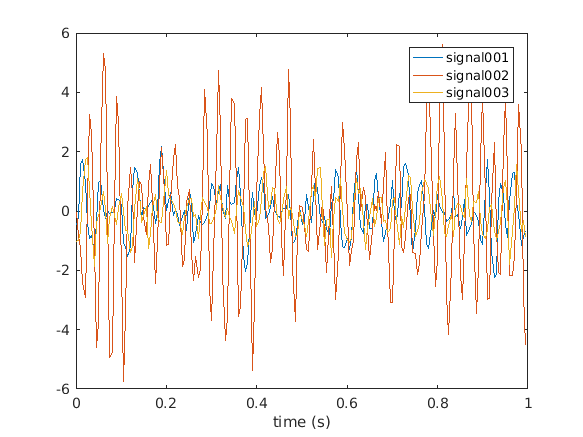
The simulated data consists of 3 channels (cfg.nsignal) in 500 trials (cfg.ntrials). You can easily visualize the data for example in the first trial using

figure
plot(data.time{1}, data.trial{1})
legend(data.label)
xlabel('time (s)')

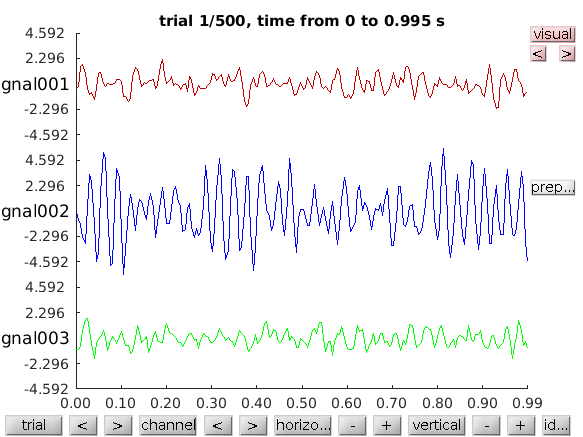
or browse through the complete data using

cfg = [];
cfg.viewmode = 'vertical';  % you can also specify 'butterfly'
ft_databrowser(cfg, data);

Computation of the multivariate autoregressive model

To be able to compute spectrally resolved Granger causality, or other frequency-domain directional measures of connectivity, we need to estimate two quantities: the spectral transfer matrix and the covariance of an autoregressive model’s residuals. We fit an autoregressive model to the data using the ft_mvaranalysis function.

For the actual computation of the autoregressive coefficients FieldTrip makes use of an implementation from third party toolboxes. At present ft_mvaranalysis supports the biosig and bsmart toolboxes for these computations.

In this tutorial we will use the bsmart toolbox. The relevant functions have been included in the FieldTrip release in the fieldtrip/external/bsmart directory. Although the exact implementations within the toolboxes differ, their outputs are comparable.

cfg         = [];
cfg.order   = 5;
cfg.toolbox = 'bsmart';
mdata       = ft_mvaranalysis(cfg, data);

mdata =
         dimord: 'chan_chan_lag'
          label: {3x1 cell}
         coeffs: [3x3x5 double]
       noisecov: [3x3 double]
            dof: 500
    fsampleorig: 200
            cfg: [1x1 struct]

The resulting variable mdata contains a description of the data in terms of a multivariate autoregressive model. For each time-lag up to the model order (cfg.order), a 3x3 matrix of coefficients is outputted. The noisecov-field contains covariance matrix of the model’s residuals.

Exercise 1

Computation of the spectral transfer function

From the autoregressive coefficients it is now possible to compute the spectral transfer matrix, for which we use ft_freqanalysis. There are several ways of computing the spectral transfer function, the parametric and the non-parametric way. We will first illustrate the parametric route:

cfg        = [];
cfg.method = 'mvar';
mfreq      = ft_freqanalysis(cfg, mdata);

mfreq =

        freq: [1x101 double]
    transfer: [3x3x101 double]
    noisecov: [3x3 double]
   crsspctrm: [3x3x101 double]
         dof: 500
        label: {3x1 cell}
       dimord: 'chan_chan_freq'
          cfg: [1x1 struct]

The resulting mfreq data structure contains the pairwise transfer function between the 3 channels for 101 frequencies.

It is also possible to compute the spectral transfer function using non-parametric spectral factorization of the cross-spectral density matrix. For this, we need a Fourier decomposition of the data. This is done in the following section.

Non-parametric computation of the cross-spectral density matrix

Some connectivity metrics can be computed from a non-parametric spectral estimate (i.e. after the application of the FFT-algorithm and conjugate multiplication to get cross-spectral densities), such as coherence, phase-locking value and phase slope index. The following part computes the Fourier-representation of the data using ft_freqanalysis.

cfg           = [];
cfg.method    = 'mtmfft';
cfg.taper     = 'dpss';
cfg.output    = 'fourier';
cfg.tapsmofrq = 2;
freq          = ft_freqanalysis(cfg, data);

freq =
            label: {3x1 cell}
           dimord: 'rpttap_chan_freq'
             freq: [1x101 double]
    fourierspctrm: [1500x3x101 double]
        cumsumcnt: [500x1 double]
        cumtapcnt: [500x1 double]
              cfg: [1x1 struct]

The resulting freq structure contains the spectral estimate for 3 tapers in each of the 500 trials (hence 1500 estimates), for each of the 3 channels and for 101 frequencies. It is not necessary to compute the cross-spectral density at this stage, because the function used in the next step, ft_connectivityanalysis, contains functionality to compute the cross-spectral density from the Fourier coefficients.

Computation and inspection of the connectivity measures

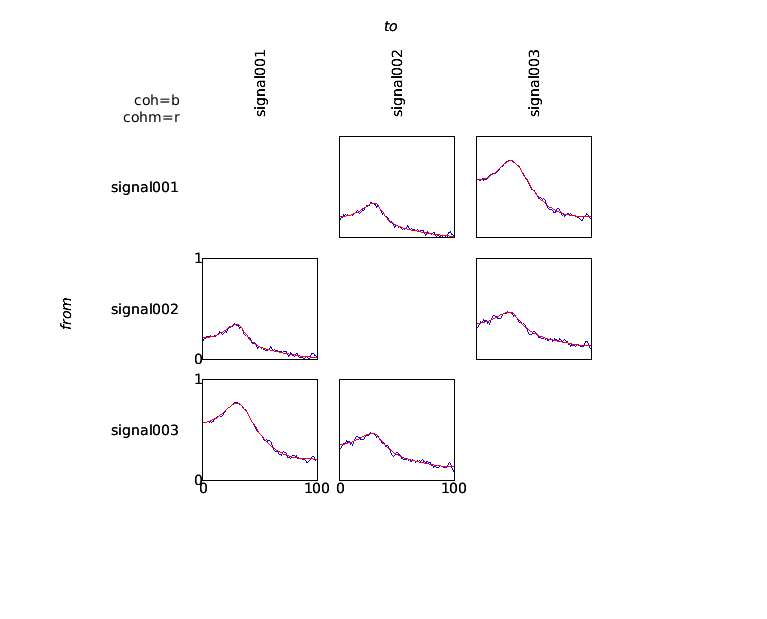
The actual computation of the connectivity metric is done by ft_connectivityanalysis. This function is transparent to the type of input data, i.e. provided the input data allows the requested metric to be computed, the metric will be calculated. Here, we provide an example for the computation and visualization of the coherence coefficient.

cfg           = [];
cfg.method    = 'coh';
coh           = ft_connectivityanalysis(cfg, freq);
cohm          = ft_connectivityanalysis(cfg, mfreq);

Subsequently, the data can be visualized using ft_connectivityplot.

cfg           = [];
cfg.parameter = 'cohspctrm';
cfg.zlim      = [0 1];
ft_connectivityplot(cfg, coh, cohm);

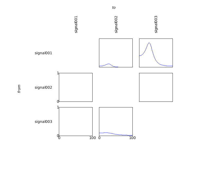
The coherence measure is a symmetric measure, which means that it does not provide information regarding the direction of information flow between any pair of signals. In order to analyze directionality in interactions, measures based on the concept of granger causality can be computed. These measures are based on an estimate of the spectral transfer matrix, which can be computed in a straightforward way from the multivariate autoregressive model fitted to the data.

cfg           = [];
cfg.method    = 'granger';
granger       = ft_connectivityanalysis(cfg, mfreq);

cfg           = [];
cfg.parameter = 'grangerspctrm';
cfg.zlim      = [0 1];
ft_connectivityplot(cfg, granger);

Exercise 2

Instead of plotting it with ft_connectivityplot, you can use the following low-level MATLAB plotting code which gives a better understanding of the numerical representation of the results.

figure
for row=1:3
for col=1:3
  subplot(3,3,(row-1)*3+col);
  plot(granger.freq, squeeze(granger.grangerspctrm(row,col,:)))
  ylim([0 1])
end
end

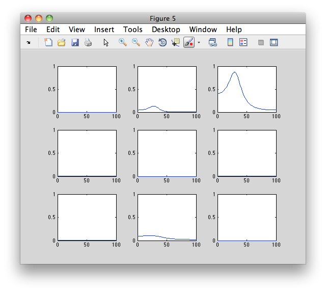
Exercise 3

Exercise 4