workshop / chieti2015 / virtualchannel /
MEG virtual channels and seed-based connectivity
Introduction
This tutorial contains hands-on material that we used for the MEG connectivity workshop in Chieti.
In this tutorial we will analyze a single-subject MEG dataset from the Human Connectome Project.
Details of the tMEG Motor task dataset
Sensory-motor processing is assessed using a task in which participants are presented with visual cues instructing the movement of either the right hand, left hand, right foot, or left foot. Movements are paced with a visual cue, which is presented in a blocked design. This task was adapted from the one developed by Buckner and colleagues (Morioka et al. 1995; Bizzi et al. 2008; Buckner et al. 2011; Yeo et al. 2011). Participants are presented with visual cues that ask them to either tap their left or right index and thumb fingers or squeeze their left or right toes. Each block of a movement type lasts 12 seconds (10 movements), and is preceded by a 3 second cue. In each of the two runs, there are 32 blocks, with 16 of hand movements (8 right and 8 left), and 16 of foot movements (8 right and 8 left). In addition, there are nine 15-second fixation blocks per run. EMG signals were used for onset of event for hand and foot movement. EMG electrode stickers are applied as shown in MEG hardware specifications and sensor locations to the skin to the lateral superior surface of the foot on the extensor digitorum brevis muscle and near the medial malleolus, also the first dorsal interosseus muscle between thumb and index finger, and the styloid process of the ulna at the wrist.
Stimulus Overview
In the Motor task, participants executed a simple hand or foot movement. The limb and the side were instructed by a visual cue, and the timing of each movement was controlled by a pacing arrow presented on the center of the screen (A, right). The paradigm included movement and rest blocks (B, right).
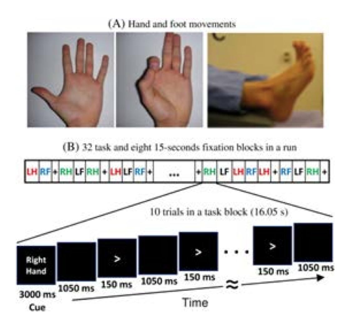
Figure Caption: A. Hand and Foot movements during the Motor Task. B. Example sequence of stimuli in a block of Right Hand motor movements.
Block/Trial Overview
Each block started with an instruction screen, indicating the side (left, right) and the limb (hand, foot) to be used by the subject in the current block. Then, 10 pacing stimuli were presented in sequence, each one instructing the participant to make a brisk movement. The pacing stimulus consisted of a small arrow in the center of the screen pointing to the side of the limb movement (left or right, above). The interval between consecutive stimuli was fixed to 1200 msec. The arrow stayed on the screen for 150 msec and for the remaining 1050 msec the screen was black.
In addition to the blocks of limb movements there were 10 interleaved resting blocks, each one of 15 sec duration. During these blocks the screen remained black. The last block was always a resting block after the last limb movement block.
The experiment was performed in 2 runs with a small break between them. The block/trial breakdown was identical in both runs. Each of the runs consisted of 42 blocks. 10 of these blocks were resting blocks, and there were 8 blocks of movement per motor effector. This yielded in total 80 movements per motor effector.
In addition to the recorded MEG channels, EMG activity was recorded from each limb. Also ECG and EOG electrodes were used to record heart- and eye movement-related electrophysiological activity.
Trigger Overview
The signal on the trigger channel consists of 2 superimposed trigger sequences. One from the Stimulus PC running the E-Prime protocol and one from a photodiode placed on the stimulus presentation screen. The trigger channel for one Motor task run is shown, top right. The photodiode was activated whenever a cueing stimulus or pacing arrow was presented on the display. It was deactivated when the display was black. The trigger value for on is 255 and the trigger value for off is 0. The photodiode trigger sequence extracted from the trigger channel of one Motor task run is shown, bottom right.
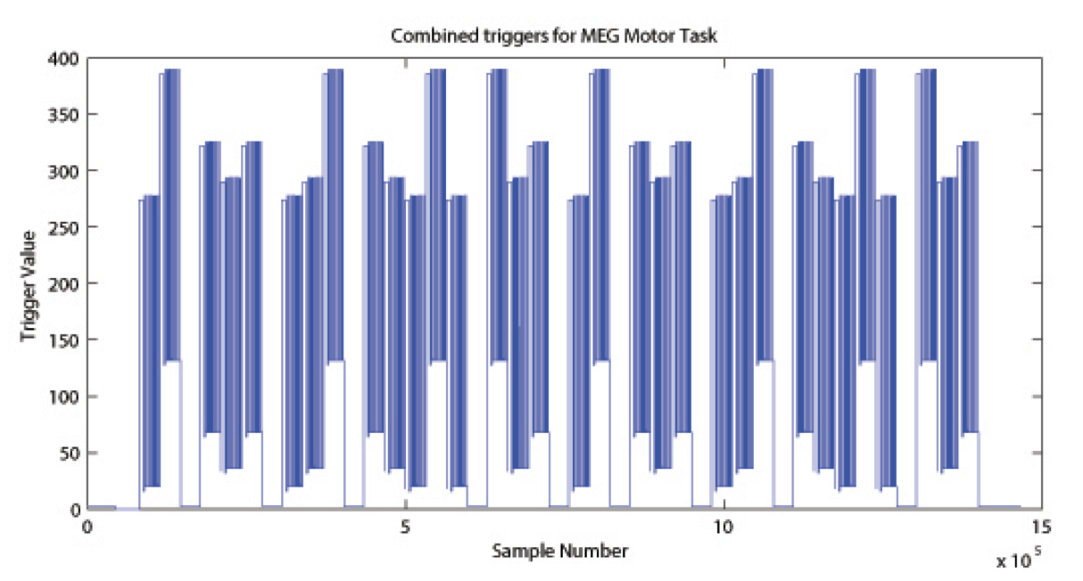
Figure Caption: Original Trigger channel sequence from one run of Motor Task. E-Prime and Photodiode triggers are superimposed.
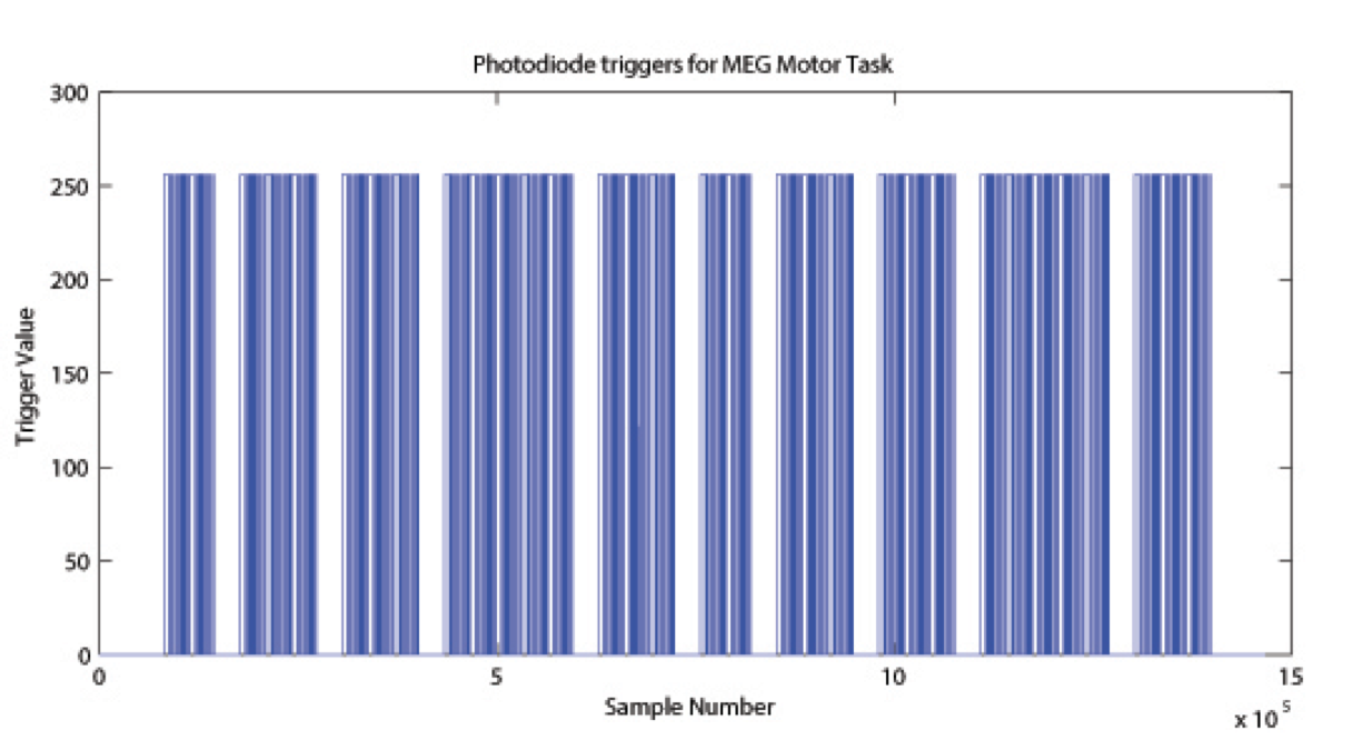
Figure Caption: Photodiode trigger sequence extracted from the Trigger channel of one Motor Task run.  The E-Prime triggers contain the information about the experimental sequence. These triggers are superimposed on the photodiode triggers, in the following description it is assumed that the photodiode triggers have been subtracted from the trigger channel so that only the triggers from the E-Prime stimulation protocol remain. Such an E-Prime trigger sequence, extracted from the trigger channel is shown, right.
For descriptions of variables (column headers) to sync the tab- delimited E-Prime output for each run see Appendix 6: Task fMRI and tMEG E-Prime Key Variables in the HCP documentation. This task contains the following events, each of which is computed against the fixation baseline.
Procedure
We start by setting up the path to the FieldTrip toolbox, to the HCP megconnectome toolbox and to the HCP data.
restoredefaultpath;
clear;
clc;

workshopdir = 'd:/';

addpath(fullfile(workshopdir, 'workshop/fieldtrip-20150909'));
ft_defaults;

addpath(genpath(fullfile(workshopdir, 'workshop/fieldtrip-20150909/template')));
addpath(genpath(fullfile(workshopdir, 'workshop/megconnectome-2.2')));
addpath(genpath(fullfile(workshopdir, 'workshop/177746')));
Load the MEG and the anatomical data
All of this has already been preprocessed and is available from http://db.humanconnectome.org.
load('177746_MEG_10-Motort_tmegpreproc_TEMG.mat')
load('177746_MEG_10-Motort_tmegpreproc_trialinfo.mat')

% the balanced gradiometer in the preprocessed data is not fully correct
% hence we use one from the unprocessed data (FIXME this is a hack)
load('177746_MEG_10-Motort_grad.mat');
data.grad = grad;

load('177746_MEG_anatomy_headmodel.mat')
tmp = load('177746_MEG_anatomy_sourcemodel_3d6mm.mat');
individual_sourcemodel3d = tmp.sourcemodel3d;
The anatomical MRI can be expressed in different coordinate systems. For some of the processing in HCP it is needed in FreeSurfer coordinates, but here we need it in 4D/BTi MEG coordinates.
individual_mri = ft_read_mri('T1w_acpc_dc_restore.nii');
hcp_read_ascii('177746_MEG_anatomy_transform.txt')
individual_mri.transform = transform.vox07mm2bti;
individual_mri.coordsys = 'bti';
Best is always to check the coordinate system of the MRI.
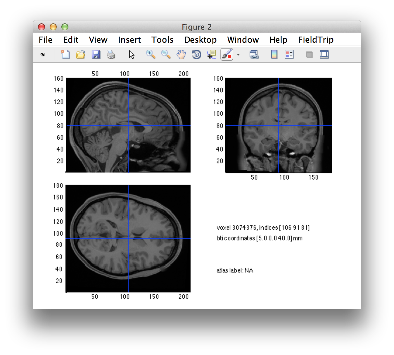
ft_sourceplot([], individual_mri);
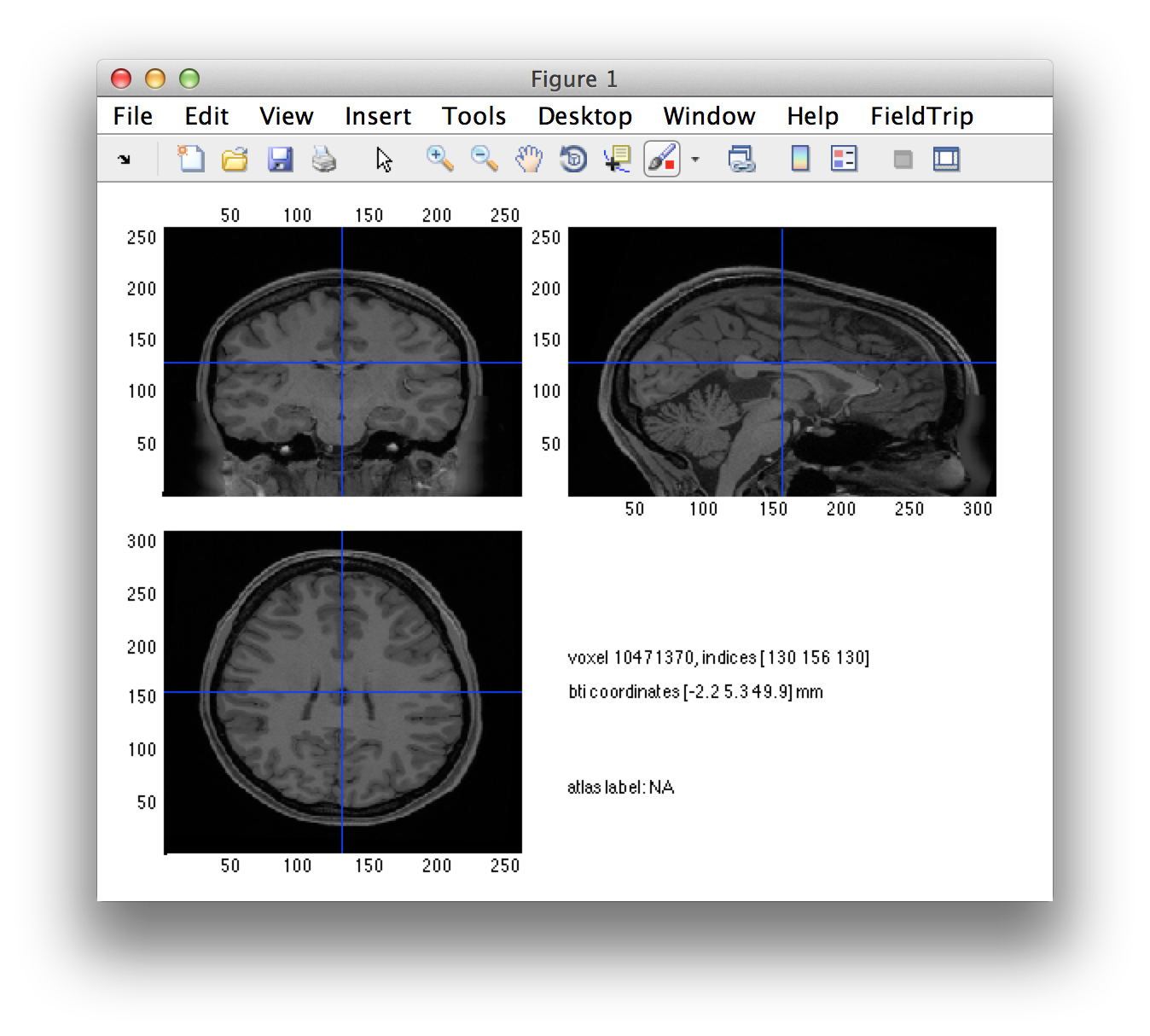
Click around in the figure and look at the “bti” head coordinates that are printed in the screen. Subsequently look up the definition of the 4D/BTi head coordinate system in this frequently asked question.
You can see that the orientation of the MRI is not as expected. Especially annoying is that it has a left-right flip. Note that each voxel’s coordinates are technically OK, but the interpretation of the figure will be easier if the MRI is resliced on a voxel grid that is aligned along the axes of the 4D/BTi coordinate system.
You might also want to read this frequently asked question which explains that there can be a difference between what your see and how the computer interprets the coordinates. You can also search google for “radiological versus neurological” representations of data.
cfg = [];
cfg.resolution = 1;
cfg.xrange = [-100 110];
cfg.yrange = [-90 90];
cfg.zrange = [-40 120];
individual_mri = ft_volumereslice(cfg, individual_mri);
Check it once more.
ft_sourceplot([], individual_mri);
% load these from the fieldtrip/template directory
template_mri = ft_read_mri('template/anatomy/single_subj_T1_1mm.nii');
tmp = load('template/sourcemodel/standard_sourcemodel3d6mm.mat');
template_sourcemodel3d = tmp.sourcemodel;
We want to visualize the various geometrical objects that we read into memory. For that we want to have them all expressed in the right coordinate system (which now has been taken care of) and in the same units.
individual_mri = ft_convert_units(individual_mri, 'mm');
individual_sourcemodel3d = ft_convert_units(individual_sourcemodel3d, 'mm');
headmodel = ft_convert_units(headmodel, 'mm');
data.grad = ft_convert_units(data.grad, 'mm');
template_mri = ft_convert_units(template_mri, 'mm');
template_sourcemodel3d = ft_convert_units(template_sourcemodel3d, 'mm');
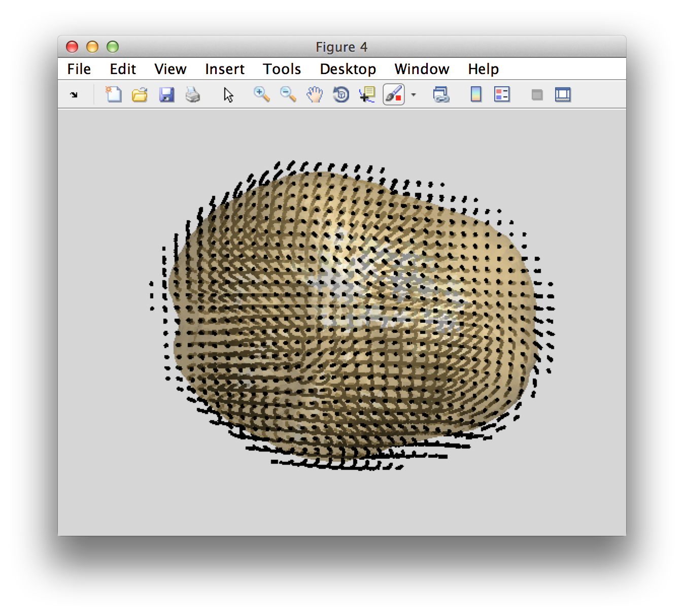
%% plot volume and channels
figure
hold on;
ft_plot_sens(data.grad, 'coil', 'yes', 'coilsize', 10);
ft_plot_headmodel(headmodel);

figure
hold on
ft_plot_headmodel(headmodel, 'facecolor', 'cortex', 'edgecolor', 'none'); alpha 0.5; camlight;
ft_plot_mesh(individual_sourcemodel3d.pos(individual_sourcemodel3d.inside, :));
ft_determine_coordsys(individual_mri, 'interactive', false); title('individual_mri')
hold on
ft_plot_sens(data.grad, 'coil', 'yes', 'coilsize', 10);
ft_plot_mesh(individual_sourcemodel3d.pos(individual_sourcemodel3d.inside, :));
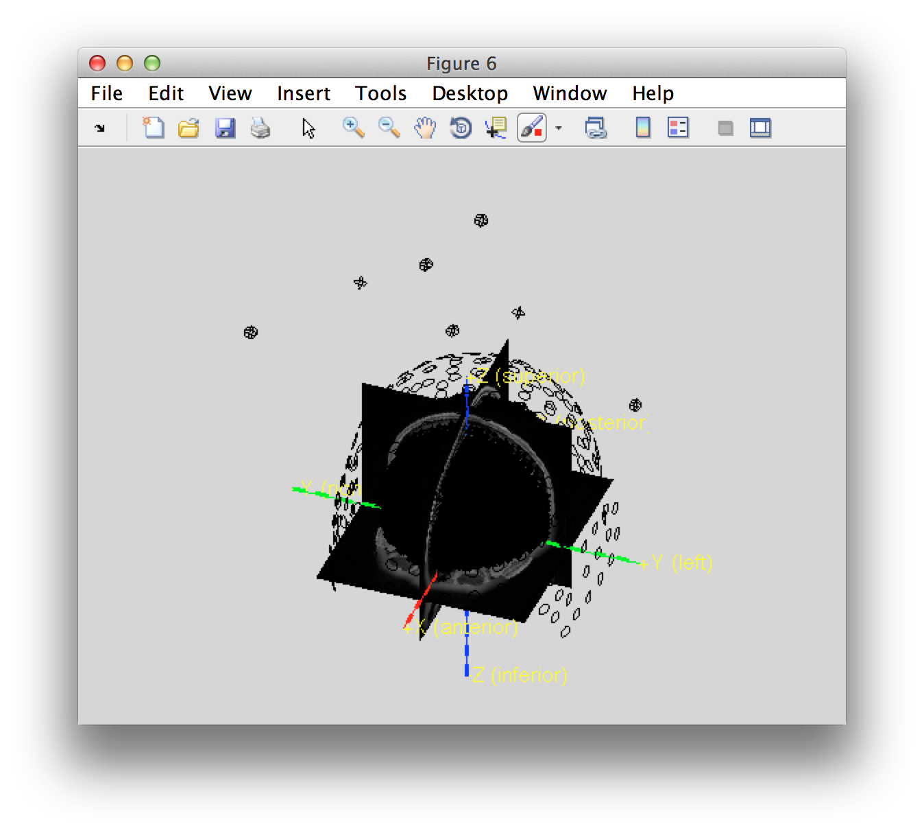
You can see that the grid locations of the source model are not exactly aligned with the axes of the coordinate systems. This is because the grid positions have been defines in MNI space and subsequently non-linearly transformed into the individual’s space according to the procedure described here.
% the figures of ft_determine_coordsys will open in their own figure
ft_determine_coordsys(template_mri, 'interactive', false); title('template_mri')
hold on
ft_plot_mesh(template_sourcemodel3d.pos(template_sourcemodel3d.inside, :));
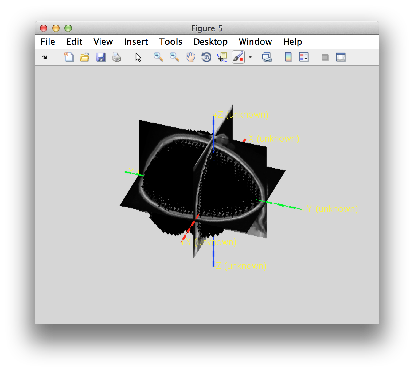
Each of the grid positions in the single-subject coordinate systems maps onto a corresponding position in the MNI coordinate system. This means that the results of this subject (and all other HCP subjects) can be directly mapped into MNI space for group comparison without the need for interpolation.
Looking for the hand movements in the MEG data
First we look at the different movements that are coded in the triggers, i.e. the movement instruction.
figure
plot(data.trialinfo(:, 2), '.')
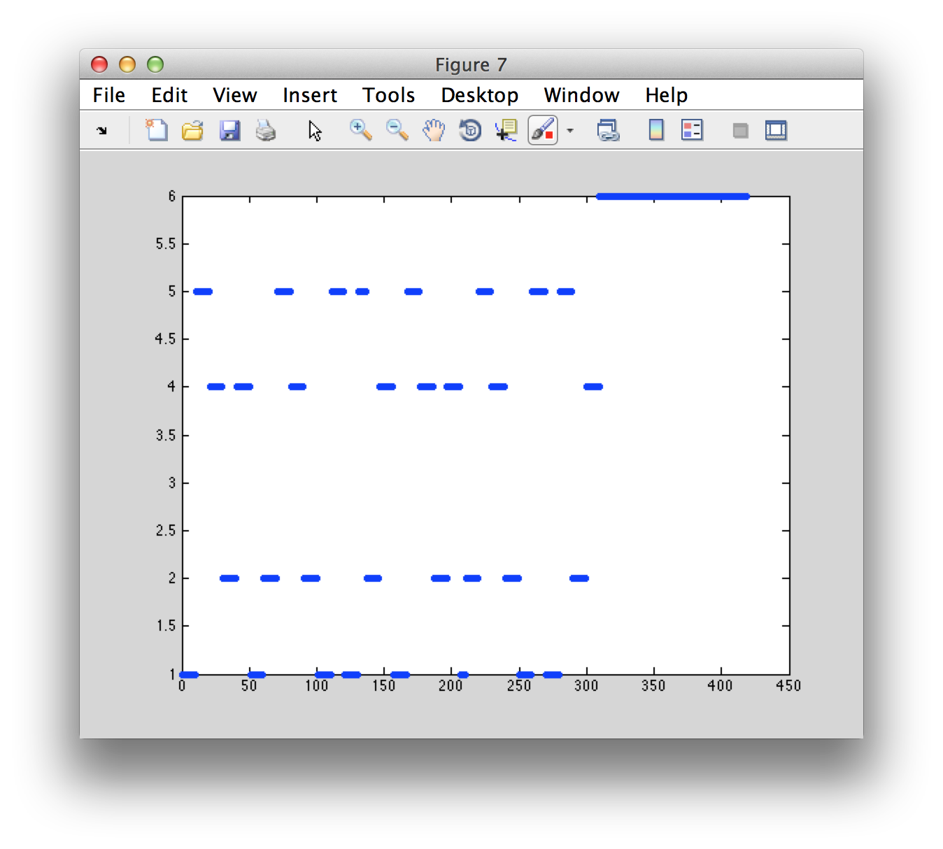
Each movement instruction is followed by a movement, which can be seen in the corresponding EMG channel. You can use ft_databrowser to browse through the subsequent trials. Each block contains multiple movements of the same hand or foot.
cfg = [];
cfg.viewmode = 'vertical';
cfg.channel = 'EMG*';
cfg.preproc.hpfilter = 'yes';
cfg.preproc.hpfreq = 30;
ft_databrowser(cfg, data);
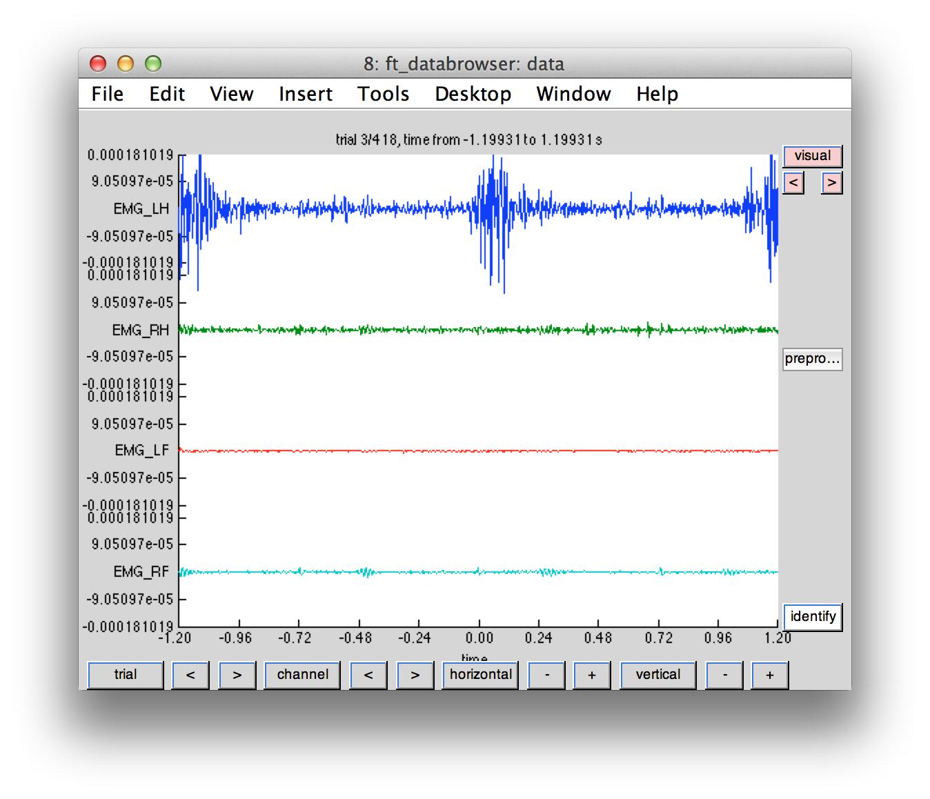
Does the mapping of the trigger codes correspond to the sequence of EMG activity?
Having done this sanity check on the data, we will make subsets for the different conditions
% 1 - Left Hand
% 2 - Left Foot
% 4 - Right Hand
% 5 - Right Foot
% 6 - Fixation

cfg = [];
cfg.trials = find(data.trialinfo(:, 2) == 1);
data_lh = ft_selectdata(cfg, data);

cfg = [];
cfg.trials = find(data.trialinfo(:, 2) == 4);
data_rh = ft_selectdata(cfg, data);

% make a shorter selection of the data around the movement
cfg = [];
cfg.toilim = [-0.75 0.75];
data_lh = ft_redefinetrial(cfg, data_lh);
data_rh = ft_redefinetrial(cfg, data_rh);
We should now only have movements of a single type, and only see a single movement in each data segment.
cfg = [];
cfg.viewmode = 'vertical';
cfg.channel = 'EMG*';
cfg.preproc.hpfilter = 'yes';
cfg.preproc.hpfreq = 30;
ft_databrowser(cfg, data_lh);

Time-frequency analysis of the MEG sensor level data
cfg = [];
cfg.channel = 'meg';
cfg.method = 'wavelet';
cfg.output = 'fourier';
cfg.keeptrials = 'yes';
cfg.foi = 1:2:60;
cfg.toi = data_lh.time{1}(1:25:end); % every 25th timepoint, approximately every 50 ms

tfr_lh = ft_freqanalysis(cfg, data_lh);
tfr_rh = ft_freqanalysis(cfg, data_rh);
Having computed the TFR, we want to visualize it. However, we computed the single-trial Fourier representation. With ft_freqdescriptives we can compute the average power
cfg = [];
tfr_lh_pow = ft_freqdescriptives(cfg, tfr_lh);
tfr_rh_pow = ft_freqdescriptives(cfg, tfr_rh);
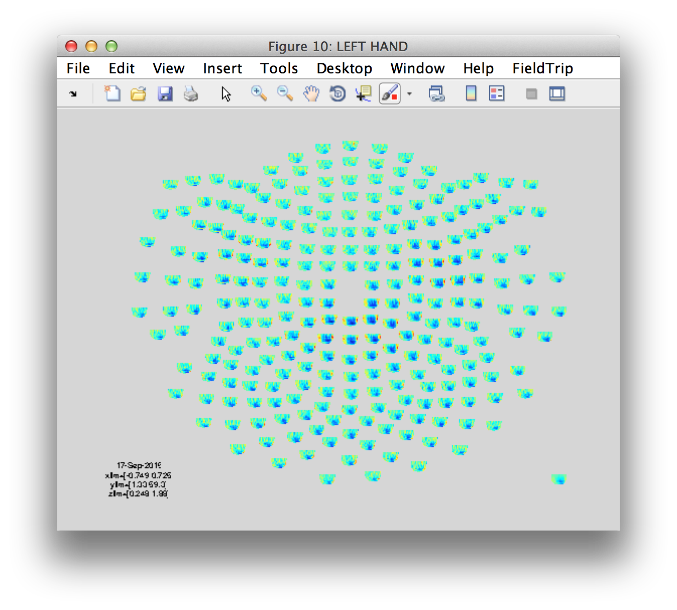
cfg = [];
cfg.baseline = [-inf -0.1];
cfg.baselinetype = 'relative';
cfg.showlabels = 'no';
cfg.layout = '4d248.lay';
% cfg.zlim = [0 2];
figure('name', 'LEFT HAND')
ft_multiplotTFR(cfg, tfr_lh_pow);
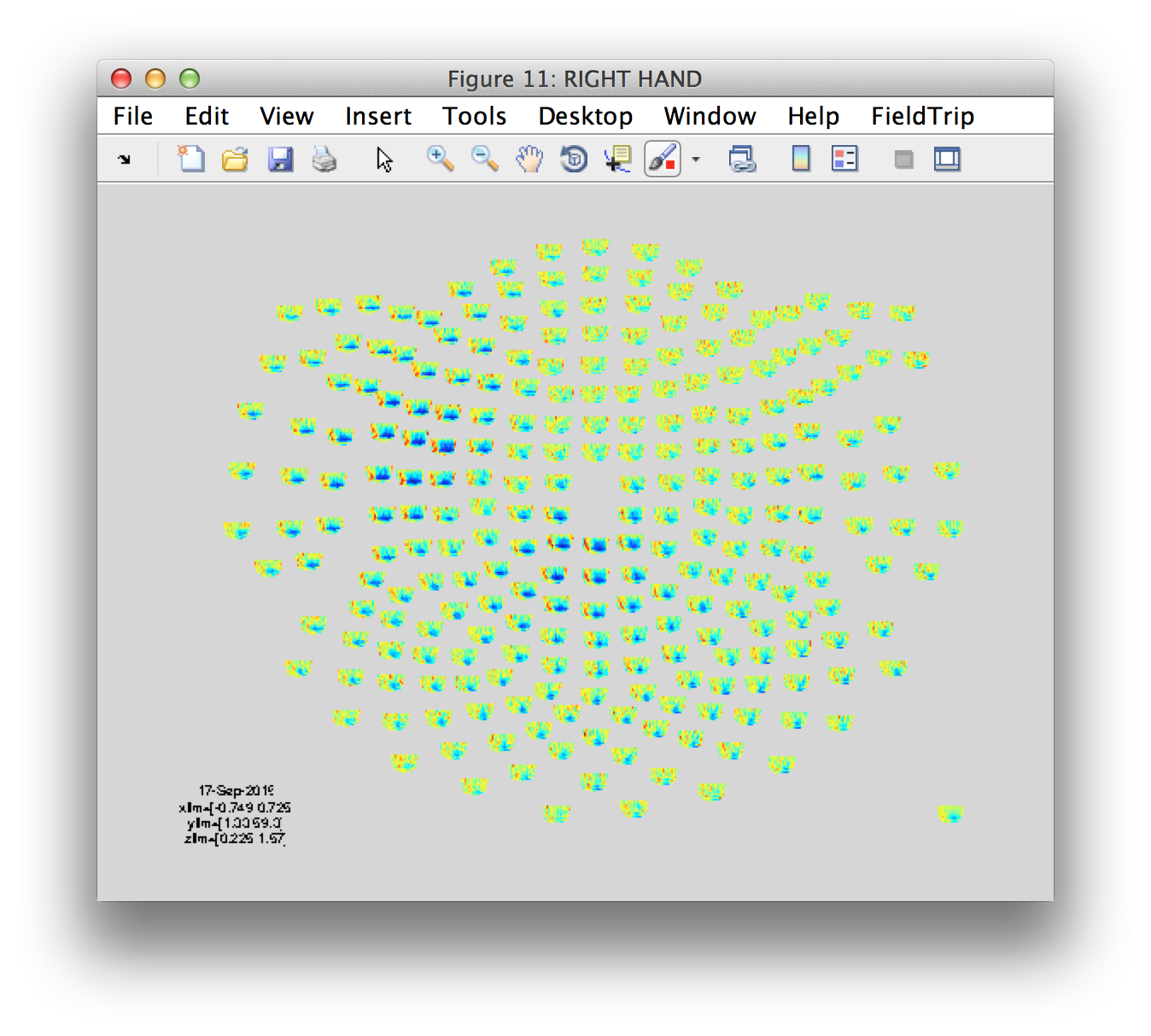
figure('name', 'RIGHT HAND')
ft_multiplotTFR(cfg, tfr_rh_pow);
We can also compute the difference between the power in the left and right-hand condition.
cfg = [];
cfg.parameter = 'powspctrm';
% cfg.operation = 'x1-x2';
cfg.operation = 'log(x1/x2)';
tfr_diff = ft_math(cfg, tfr_lh_pow, tfr_rh_pow);

cfg = [];
cfg.layout = '4d248.lay';
cfg.zlim = 'maxabs';
figure('name', 'DIFFERENCE')
ft_multiplotTFR(cfg, tfr_diff);

You should use the interactive functionality of the ft_multiplotTFR figures. Click in the figures to identify the time, frequency and channel selections that show interesting effects.
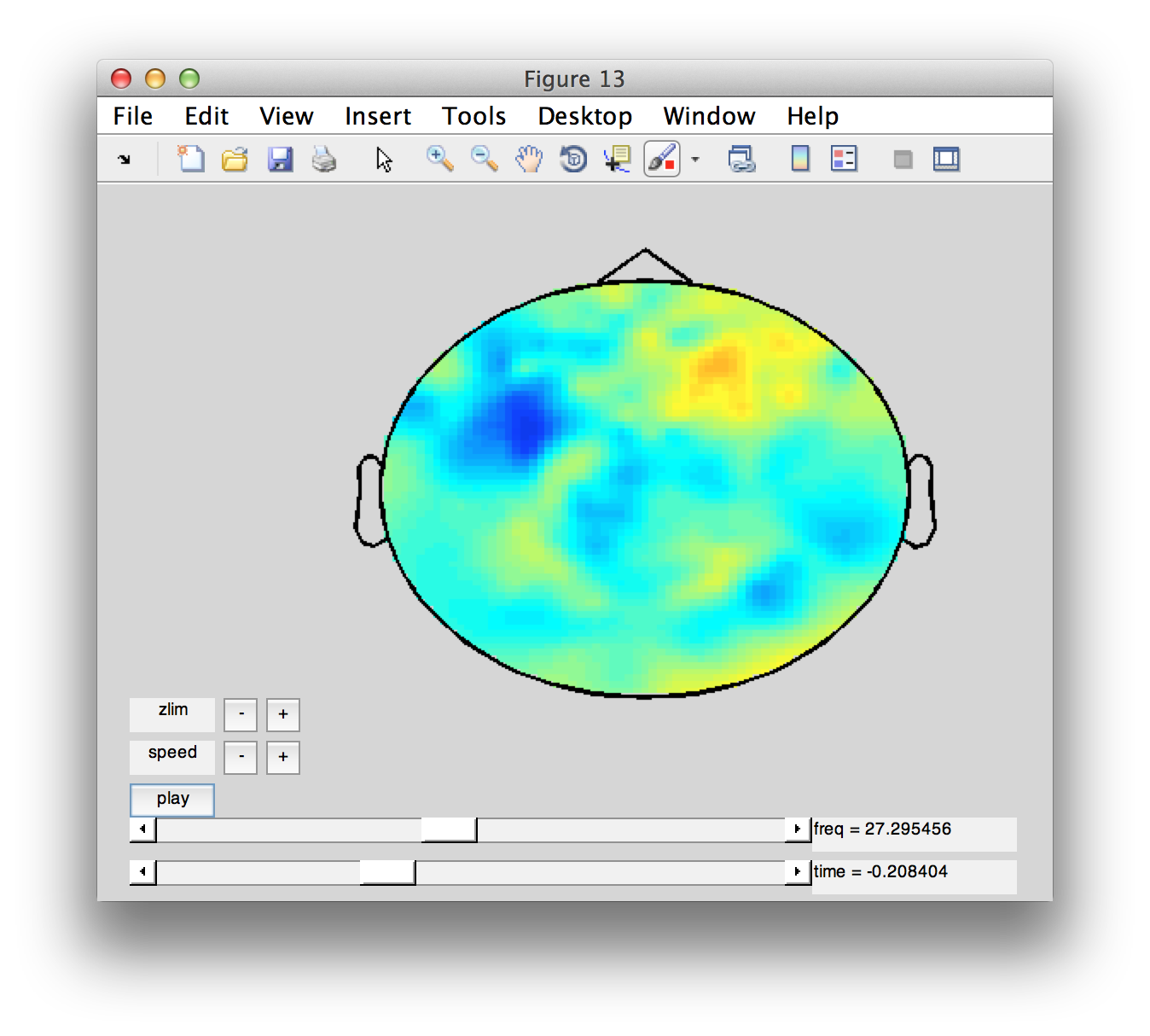
Another way of looking at the dynamics in this channel-time-frequency representation is by making a movi
figure;
cfg = [];
cfg.zlim = 'maxabs';
cfg.layout = '4d248.lay';
ft_movieplotTFR(cfg, tfr_diff);
Localize the beta band activity
Around the movement there is a clear differential beta-band effect over bilateral sensory-motor areas. We can zoom in on this effect using DICS as frequency domain source reconstruction.
Create the lead field, i.e. the forward model
cfg = [];
cfg.grid = individual_sourcemodel3d;
cfg.headmodel = headmodel;

cfg.grad = data_rh.grad;
cfg.channel = ft_channelselection('MEG', data_rh.label);
cfg.reducerank = 2;
cfg.normalize = 'yes';
leadfield = ft_prepare_leadfield(cfg);
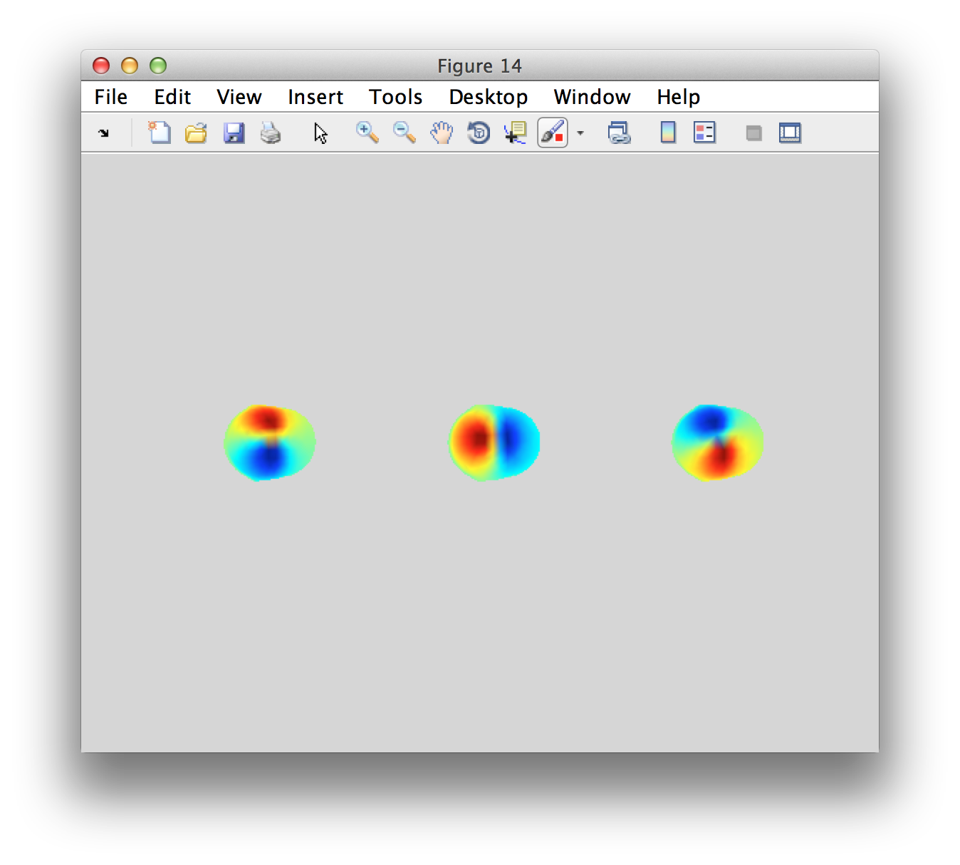
Usually we would not look at the forward solution, i.e. the lead fields. But the quality of the forward model and lead fields influences the quality of the source-level estimate that we will get. Let’s visualize the lead field for the most superior source close to the vertex.
selchan = match_str(data.grad.label, leadfield.label);
% selpos = find(leadfield.inside, 1, 'first');
selpos = find(leadfield.inside, 1, 'last');
figure
subplot(1,3,1); ft_plot_topo3d(data_rh.grad.chanpos(selchan,:), leadfield.leadfield{selpos}(:,1));
subplot(1,3,2); ft_plot_topo3d(data_rh.grad.chanpos(selchan,:), leadfield.leadfield{selpos}(:,2));
subplot(1,3,3); ft_plot_topo3d(data_rh.grad.chanpos(selchan,:), leadfield.leadfield{selpos}(:,3));
Rather than doing the source reconstruction on the wavelet decomposed data, we can zoom in and concentrate the spectral estimation in the exact time-frequency window of interest (following movement, around 20 Hz).
% make a selection of 500ms directly following movement
cfg = [];
cfg.toilim = [0 0.5];
data_rh_sel = ft_redefinetrial(cfg, data_rh);
data_lh_sel = ft_redefinetrial(cfg, data_lh);

% do a non-timeresolved spectral estimate at 20 Hz with 7 Hz smoothing in both directions (i.e. smoothing from 13-27 Hz).
cfg = [];
cfg.channel = 'meg';
cfg.method = 'mtmfft';
cfg.output = 'powandcsd';
cfg.foilim = [20 20];
cfg.tapsmofrq = 7;
tfr_rh_sel = ft_freqanalysis(cfg, data_rh_sel);
tfr_lh_sel = ft_freqanalysis(cfg, data_lh_sel);
Using the cross-spectral density matrix, we can do the beamformer estimate of the power at each of the grid locations in the source model.
cfg = [];
cfg.method = 'dics';
cfg.frequency = 20;
cfg.grid = leadfield;
cfg.headmodel = headmodel;
cfg.dics.realfilter = 'yes';
cfg.dics.projectnoise = 'yes';
cfg.dics.lambda = '10%';
dics_rh = ft_sourceanalysis(cfg, tfr_rh_sel);
dics_lh = ft_sourceanalysis(cfg, tfr_lh_sel);
The source reconstruction contains the power at each grid location, but also the noise. Explore the structure, especially “source.avg”. Can you find the power and the noise estimate? Why is the estimate not computed for all grid locations?
The beamformer can be biassed to deep locations, since noise gets projected to locations with a very small lead field (deep inside the head). The neural activity index allows for compensating for the depth bias, as explained here.
Using ft_sourcedescriptives we compute the neural activity index, i.e. the ratio between power and the projected noise estimate.
cfg = [];
dics_lh = ft_sourcedescriptives(cfg, dics_lh);
dics_rh = ft_sourcedescriptives(cfg, dics_rh);
Since we have the left- and right-hand conditions, which have the same depth bias, we can also compute a contrast (i.e. difference) between the conditions.
cfg = [];
cfg.parameter = 'pow';
cfg.operation = 'log(x1/x2)';
dics_diff = ft_math(cfg, dics_lh, dics_rh);
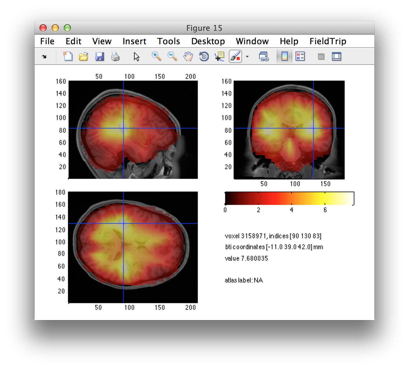
Following interpolation of the (non-uniform grid) source reconstructed data onto the individual’s MRI, we can visualize the distribution of the source estimate.
cfg = [];
cfg.parameter = 'all';
dics_lh_int = ft_sourceinterpolate(cfg, dics_lh, individual_mri);
dics_rh_int = ft_sourceinterpolate(cfg, dics_rh, individual_mri);
dics_diff_int = ft_sourceinterpolate(cfg, dics_diff, individual_mri);

cfg = [];
cfg.funparameter = 'nai'; % or 'pow'
cfg.anaparameter = 'anatomy';
ft_sourceplot(cfg, dics_lh_int);
ft_sourceplot(cfg, dics_rh_int);

cfg = [];
cfg.funparameter = 'pow';
cfg.anaparameter = 'anatomy';
% cfg.location = [181 138 125];
% cfg.locationcoordinates = 'voxel';
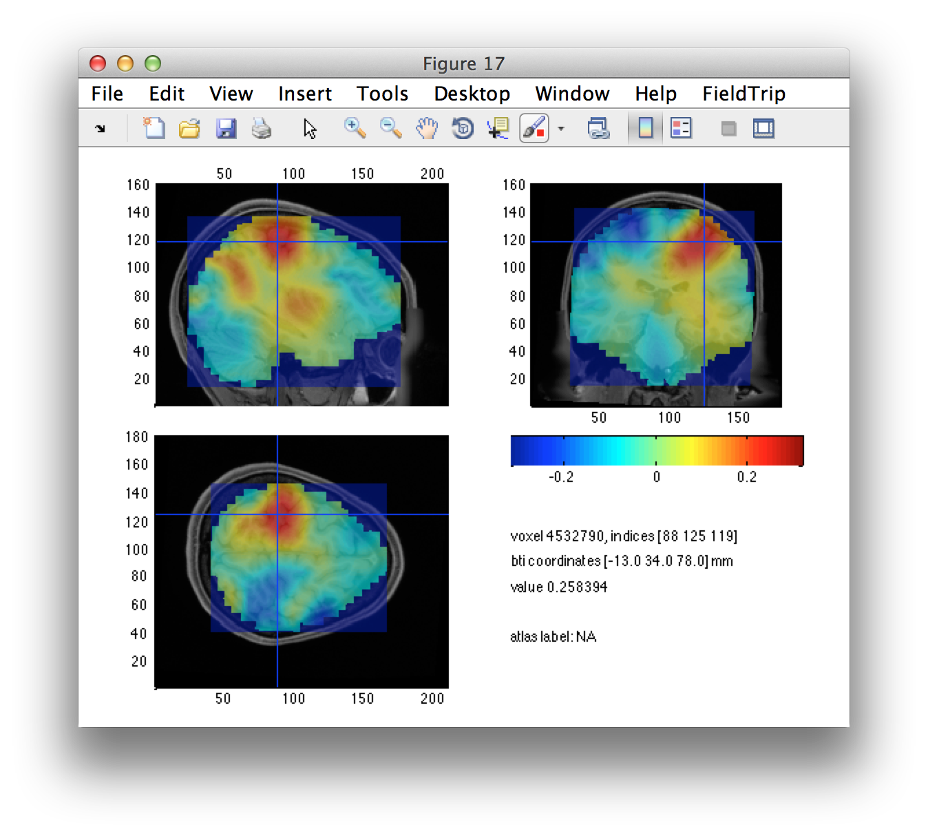
ft_sourceplot(cfg, dics_diff_int);
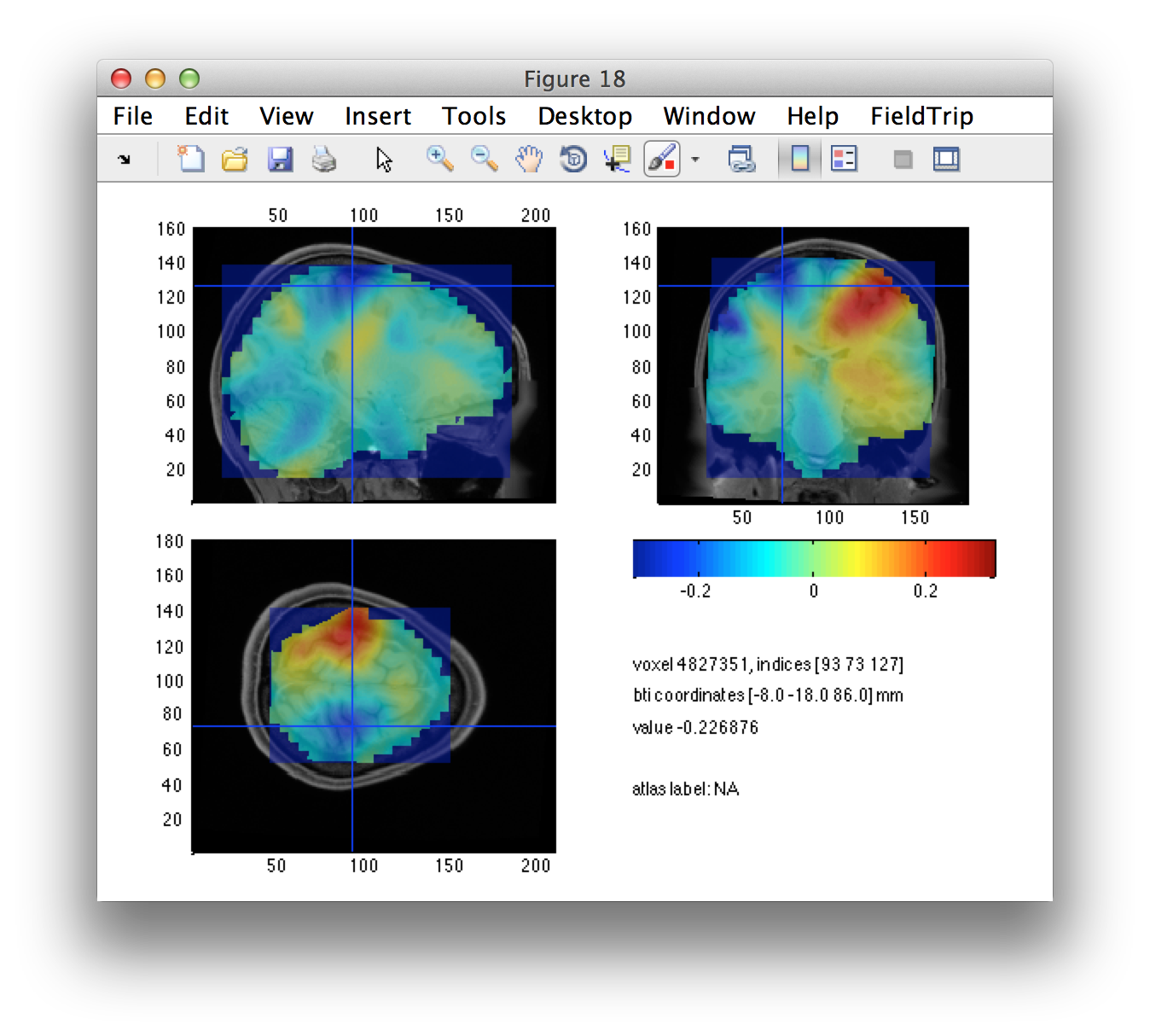
Estimate seed based connectivity
The left/right source-level contrast image gives us a suggestion of the left and right motor cortices. Using the interactive option of ft_sourceplot, we can click around in the figure and identify the voxel coordinates of the peak in both hemispheres.
We can define the seeds, expressed in voxels. Subsequently we have to convert these from voxel to BTi coordinates.
lh_seed_vox = [88   125   119]; %% left hemisphere
rh_seed_vox = [93    73   127]; %% right hemisphere

lh_seed_pos = ft_warp_apply(individual_mri.transform, lh_seed_vox, 'homogeneous');
rh_seed_pos = ft_warp_apply(individual_mri.transform, rh_seed_vox, 'homogeneous');
Note that we could also have read the head coordinates directly from the source plot figure.
We also define a seed region in the midline as a control region. We would not expect any differential activity here.
ml_seed_pos = (lh_seed_pos + rh_seed_pos)/2;
Let’s check that the seed locations match with the regions that we have identified as interesting.
cfg = [];
cfg.funparameter = 'pow';
cfg.anaparameter = 'anatomy';
cfg.locationcoordinates = 'head';
cfg.location = lh_seed_pos;
ft_sourceplot(cfg, dics_diff_int);
cfg.location = rh_seed_pos;
ft_sourceplot(cfg, dics_diff_int);
cfg.location = ml_seed_pos;
ft_sourceplot(cfg, dics_diff_int);

Perform timelock analysis
Rather than continuing in the frequency domain at a specific frequency, we will return to the original channel level data. Using the LCMV beamformer, we can compute virtual channel time series at the locations of interest. This requires the data covarianc
cfg = [];
cfg.channel = 'meg';
cfg.covariance = 'yes'; % compute the covariance for single trials, then average
cfg.preproc.bpfilter = 'yes';
cfg.preproc.bpfreq = [5 75];
cfg.preproc.demean = 'yes';
cfg.preproc.baselinewindow = [-inf 0]; % baseline correction
cfg.keeptrials = 'no';
cfg.vartrllength = 2;

timelock_rh = ft_timelockanalysis(cfg, data_rh);
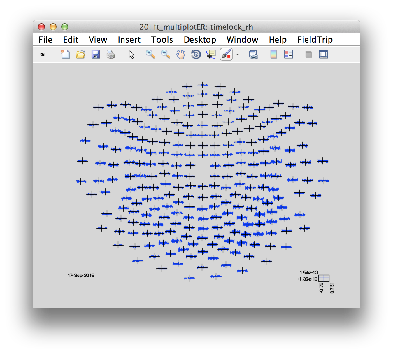
Let’s look at the distribution of the movement-locked ER
cfg = [];
cfg.layout = '4d248.lay';
figure
ft_multiplotER(cfg, timelock_rh);
With the covariance and the forward model for the specific seed points, we can compute the spatial filter. Since there are only three locations now, there is no need to pre-compute the lead field.
cfg = [];
cfg.headmodel = headmodel;
cfg.senstype = 'meg';
cfg.method = 'lcmv';
cfg.keepleadfield = 'yes';
cfg.lcmv.keepfilter = 'yes';
cfg.lcmv.projectmom = 'yes';
cfg.lcmv.lambda = '10%';
cfg.units = 'mm';

cfg.sourcemodel.pos = [
lh_seed_pos
rh_seed_pos
ml_seed_pos
];

lcmv_rh = ft_sourceanalysis(cfg, timelock_rh);
Look at the source structure, again in “source.avg”. Can you find the representation of the spatial filter?
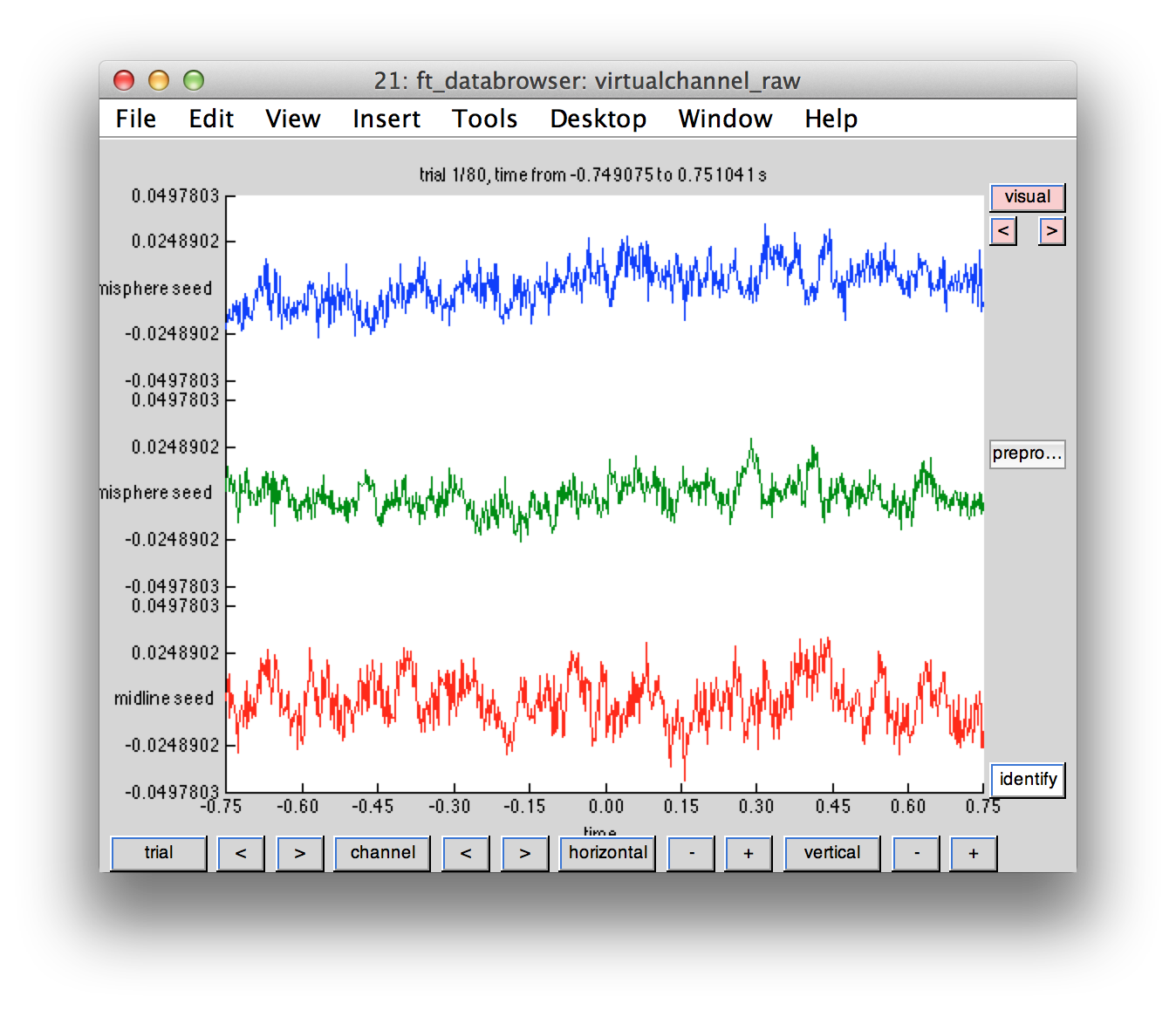
Using the spatial filters, we construct single-trial virtual channel time series. This results in three channels. We can represent this data in the same fashion as the original raw data.
cfg = [];
cfg.channel = 'meg';
data_rh_meg = ft_selectdata(cfg, data_rh);

virtualchannel_raw = [];
virtualchannel_raw.label{1, 1} = 'left hemisphere seed';
virtualchannel_raw.label{2, 1} = 'right hemisphere seed';
virtualchannel_raw.label{3, 1} = 'midline seed';
for i = 1:size(data_rh_meg.trial, 2)
virtualchannel_raw.time{i} = data_rh_meg.time{i};
virtualchannel_raw.trial{i}(1, :) = lcmv_rh.avg.filter{1} * data_rh_meg.trial{i}(:, :);
virtualchannel_raw.trial{i}(2, :) = lcmv_rh.avg.filter{2} * data_rh_meg.trial{i}(:, :);
virtualchannel_raw.trial{i}(3, :) = lcmv_rh.avg.filter{3} * data_rh_meg.trial{i}(:, :);
end
Just like MEG channel level data, we can plot the time courses of the virtual channel
cfg = [];
cfg.viewmode = 'vertical';
ft_databrowser(cfg, virtualchannel_raw);
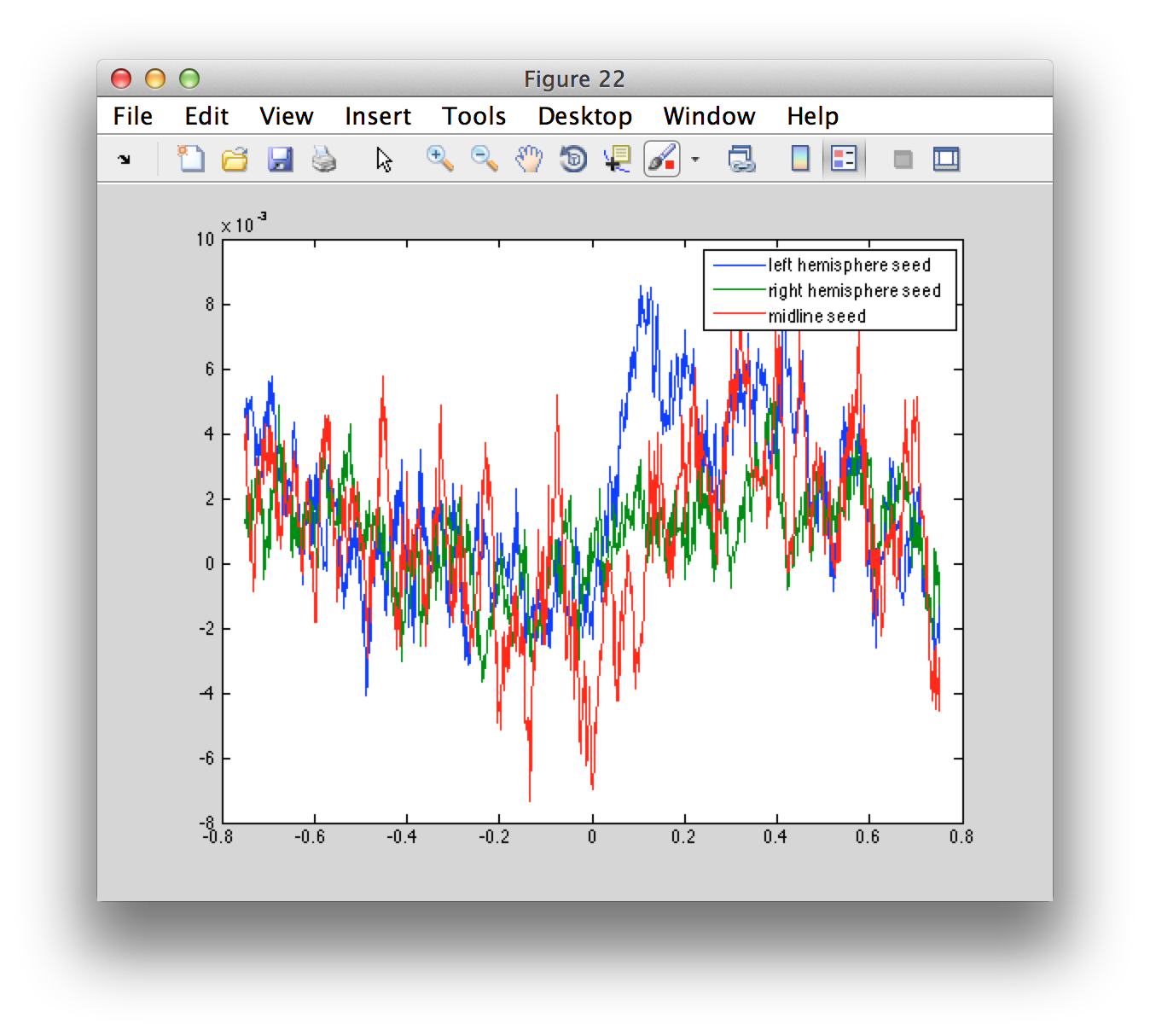
We can also compute the source-level ERF
cfg = [];
cfg.preproc.demean = 'yes';
cfg.preproc.baselinewindow = [-0.6 -0.1];
virtualchannel_avg = ft_timelockanalysis(cfg, virtualchannel_raw);

figure
plot(virtualchannel_avg.time, virtualchannel_avg.avg)
legend(virtualchannel_avg.label);
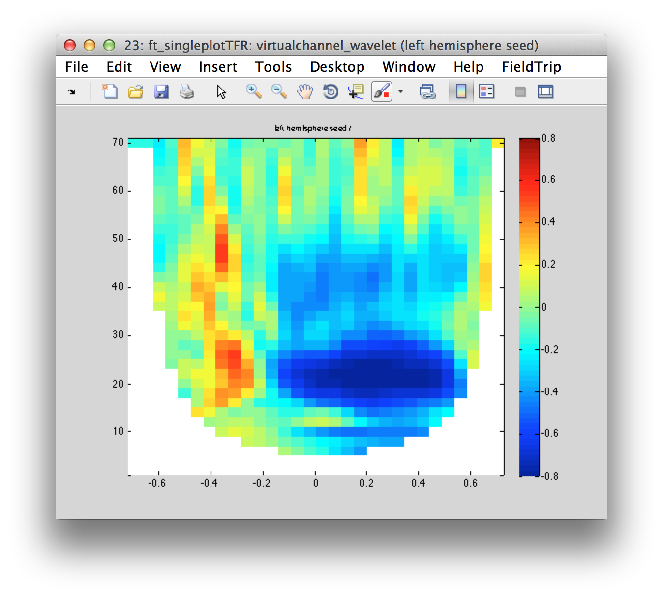
and we can compute the source-level time-frequency representation of the virtual channel data
cfg = [];
cfg.output = 'powandcsd';
cfg.foi = 2:2:70;
cfg.toi = -0.7:0.05:0.7;
cfg.method = 'mtmconvol';
cfg.taper = 'hanning';
cfg.t_ftimwin = 7./cfg.foi; % 7 cycles per time window
virtualchannel_wavelet = ft_freqanalysis(cfg, virtualchannel_raw);
cfg = [];
cfg.baselinetype = 'relchange';
cfg.baseline = [-0.6 -0.1];
cfg.zlim = [-0.8 0.8];
cfg.channel = {'left hemisphere seed'};
figure; ft_singleplotTFR(cfg, virtualchannel_wavelet);
cfg.channel = {'right hemisphere seed'};
figure; ft_singleplotTFR(cfg, virtualchannel_wavelet);
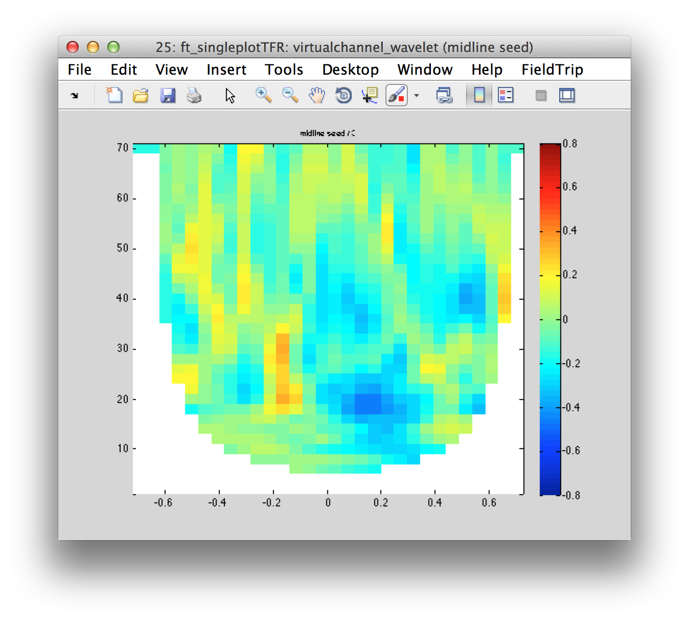
cfg.channel = {'midline seed'};
figure; ft_singleplotTFR(cfg, virtualchannel_wavelet);

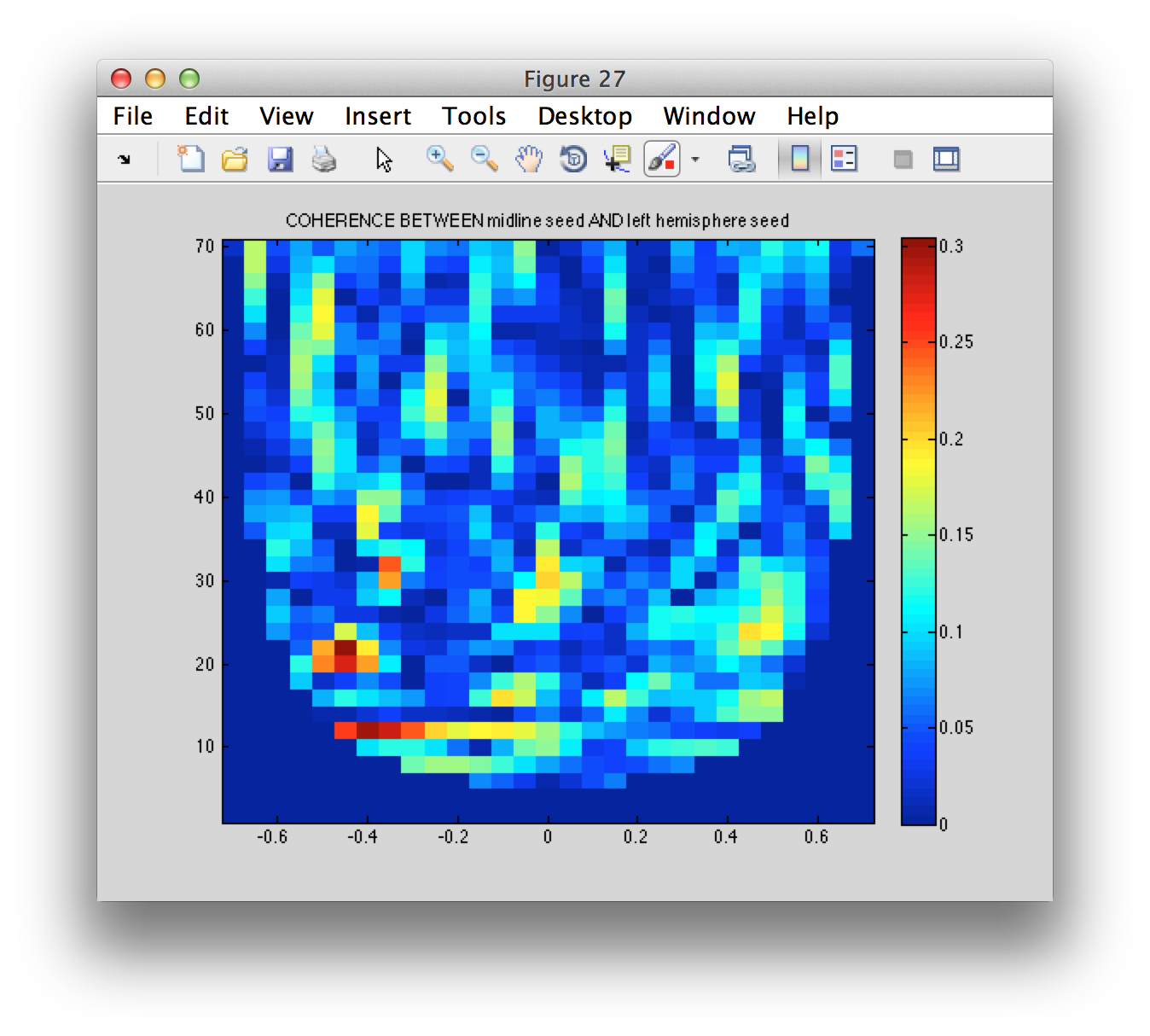
Virtual channel connectivity
The virtual channel time series seem to be consistent with what we expect to happen in motor cortex around a movement. Using the time-frequency estimate, we can compute the imaginary coherence between the three seed region
cfg = [];
cfg.method = 'coh';
cfg.complex = 'absimag';
coherence = ft_connectivityanalysis(cfg, virtualchannel_wavelet);

figure
imagesc(coherence.time, coherence.freq, squeeze(coherence.cohspctrm(1, :, :)));
title(sprintf('COHERENCE BETWEEN %s AND %s', coherence.labelcmb{1,1}, coherence.labelcmb{1,2}))
colorbar
axis xy

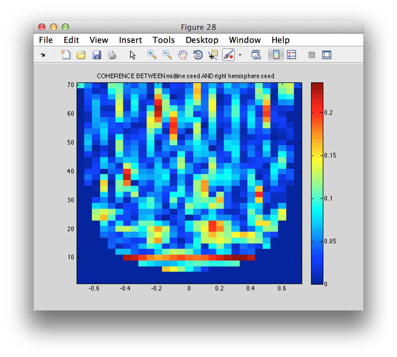
figure
imagesc(coherence.time, coherence.freq, squeeze(coherence.cohspctrm(2, :, :)));
title(sprintf('COHERENCE BETWEEN %s AND %s', coherence.labelcmb{2,1}, coherence.labelcmb{2,2}))
colorbar
axis xy
figure
imagesc(coherence.time, coherence.freq, squeeze(coherence.cohspctrm(3, :, :)));
title(sprintf('COHERENCE BETWEEN %s AND %s', coherence.labelcmb{3,1}, coherence.labelcmb{3,2}))
colorbar
axis xy
There are many more connectivity methods available in ft_connectivityanalysis. Try out some of the others.