workshop / chieti2015 / wholebrain /
MEG whole-brain connectivity
Introduction
This tutorial contains hands-on material that we used for the MEG connectivity workshop in Chieti.
In this tutorial we will analyze a single-subject MEG dataset from the Human Connectome Project.
Details of the tMEG Motor task dataset
Sensory-motor processing is assessed using a task in which participants are presented with visual cues instructing the movement of either the right hand, left hand, right foot, or left foot. Movements are paced with a visual cue, which is presented in a blocked design. This task was adapted from the one developed by Buckner and colleagues (Morioka et al. 1995; Bizzi et al. 2008; Buckner et al. 2011; Yeo et al. 2011). Participants are presented with visual cues that ask them to either tap their left or right index and thumb fingers or squeeze their left or right toes. Each block of a movement type lasts 12 seconds (10 movements), and is preceded by a 3 second cue. In each of the two runs, there are 32 blocks, with 16 of hand movements (8 right and 8 left), and 16 of foot movements (8 right and 8 left). In addition, there are nine 15-second fixation blocks per run. EMG signals were used for onset of event for hand and foot movement. EMG electrode stickers are applied as shown in MEG hardware specifications and sensor locations to the skin to the lateral superior surface of the foot on the extensor digitorum brevis muscle and near the medial malleolus, also the first dorsal interosseus muscle between thumb and index finger, and the styloid process of the ulna at the wrist.
Stimulus Overview
In the Motor task, participants executed a simple hand or foot movement. The limb and the side were instructed by a visual cue, and the timing of each movement was controlled by a pacing arrow presented on the center of the screen (A, right). The paradigm included movement and rest blocks (B, right).
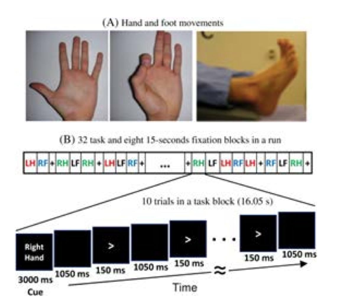
Figure Caption: A. Hand and Foot movements during the Motor Task. B. Example sequence of stimuli in a block of Right Hand motor movements.
Block/Trial Overview
Each block started with an instruction screen, indicating the side (left, right) and the limb (hand, foot) to be used by the subject in the current block. Then, 10 pacing stimuli were presented in sequence, each one instructing the participant to make a brisk movement. The pacing stimulus consisted of a small arrow in the center of the screen pointing to the side of the limb movement (left or right, above). The interval between consecutive stimuli was fixed to 1200 msec. The arrow stayed on the screen for 150 msec and for the remaining 1050 msec the screen was black.
In addition to the blocks of limb movements there were 10 interleaved resting blocks, each one of 15 sec duration. During these blocks the screen remained black. The last block was always a resting block after the last limb movement block.
The experiment was performed in 2 runs with a small break between them. The block/trial breakdown was identical in both runs. Each of the runs consisted of 42 blocks. 10 of these blocks were resting blocks, and there were 8 blocks of movement per motor effector. This yielded in total 80 movements per motor effector.
In addition to the recorded MEG channels, EMG activity was recorded from each limb. Also ECG and EOG electrodes were used to record heart- and eye movement-related electrophysiological activity.
Trigger Overview
The signal on the trigger channel consists of 2 superimposed trigger sequences. One from the Stimulus PC running the E-Prime protocol and one from a photodiode placed on the stimulus presentation screen. The trigger channel for one Motor task run is shown, top right. The photodiode was activated whenever a cueing stimulus or pacing arrow was presented on the display. It was deactivated when the display was black. The trigger value for on is 255 and the trigger value for off is 0. The photodiode trigger sequence extracted from the trigger channel of one Motor task run is shown, bottom right.
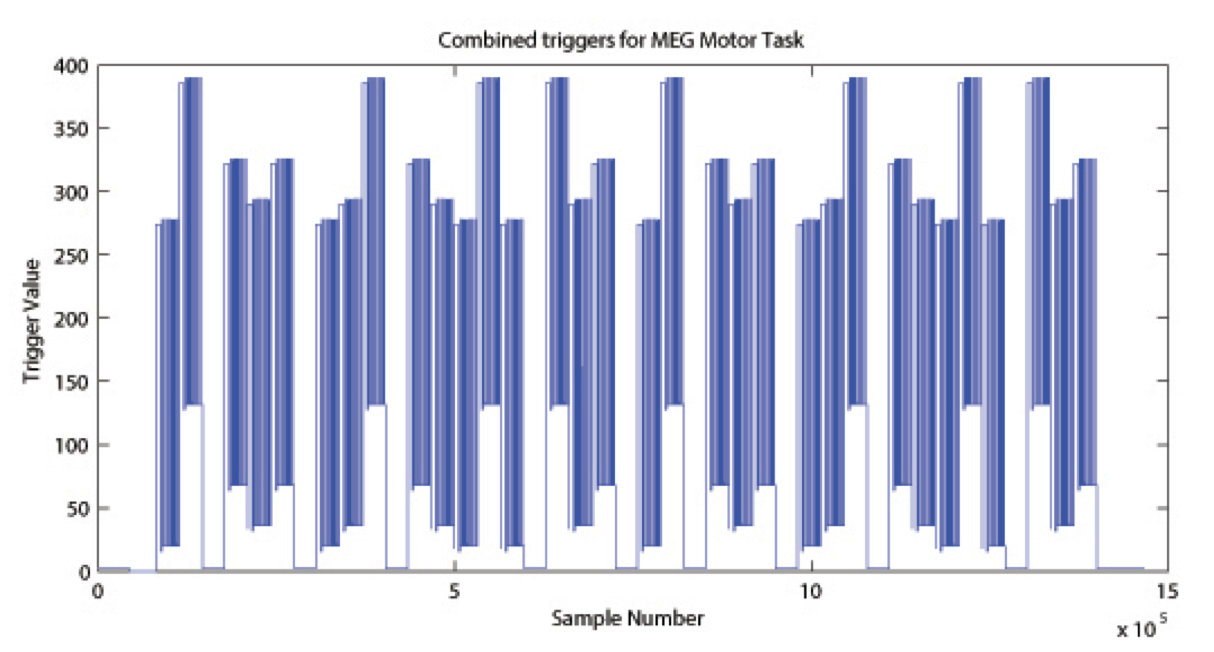
Figure Caption: Original Trigger channel sequence from one run of Motor Task. E-Prime and Photodiode triggers are superimposed.
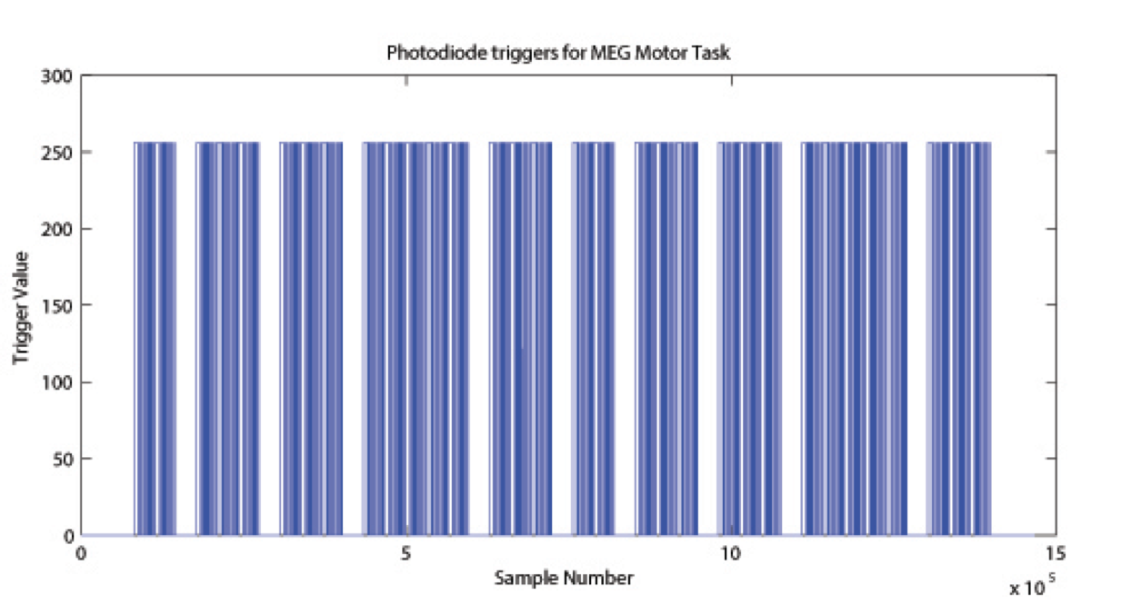
Figure Caption: Photodiode trigger sequence extracted from the Trigger channel of one Motor Task run.  The E-Prime triggers contain the information about the experimental sequence. These triggers are superimposed on the photodiode triggers, in the following description it is assumed that the photodiode triggers have been subtracted from the trigger channel so that only the triggers from the E-Prime stimulation protocol remain. Such an E-Prime trigger sequence, extracted from the trigger channel is shown, right.
For descriptions of variables (column headers) to sync the tab- delimited E-Prime output for each run see Appendix 6: Task fMRI and tMEG E-Prime Key Variables in the HCP documentation. This task contains the following events, each of which is computed against the fixation baseline.
This tutorial follows on the MEG virtual channels and seed-based connectivity tutorial and continues with the data that has already partially been computed there.
Procedure
We start by setting up the path to the FieldTrip toolbox, to the HCP megconnectome toolbox and to the HCP data.
restoredefaultpath;
clear;
clc;

addpath('/Volumes/SEAGATE 2TB/workshop/fieldtrip-20150909');
ft_defaults;
addpath(genpath('/Volumes/SEAGATE 2TB/workshop/fieldtrip-20150909/template'));
addpath(genpath('/Volumes/SEAGATE 2TB/workshop/megconnectome-2.2'));
addpath(genpath('/Volumes/SEAGATE 2TB/workshop/177746'));
Most data has already been prepared in the previous tutorial, here we just load the relevant .mat files.
load data_rh
load headmodel
load leadfield
load freq
load lh_seed_pos
load rh_seed_pos
load ml_seed_pos
load individual_mri
Whole brain connectivity, starting at a seed location
Previously we computed the time-frequency representation over the full time and frequency range, and we computed with “mtmfft” the multi-tapered spectral representation at a single time-frequency point. We can also use wavelets to obtain the spectral estimate at a single time-frequency point.
cfg = [];
cfg.channel = 'meg';
cfg.method = 'wavelet';
cfg.output = 'fourier';
cfg.keeptrials = 'yes';
cfg.foi = 20;
cfg.toi = 0.100; % just following movement onset
freq = ft_freqanalysis(cfg, data_rh);
The have pre-computed the lead field for a full 3-D grid with source locations. We can project the spectral estimate from the channel-level into the source-level using the “pcc” method. This is a modification of the original DICS method that allows post-hoc computation of various connectivity measures.
cfg = [];
cfg.headmodel = headmodel;
cfg.grid = leadfield;
cfg.method = 'pcc';
cfg.pcc.fixedori = 'yes';

source = ft_sourceanalysis(cfg, freq);
The source level data now contains the complex-values spectral estimate at each grid location.
figure
plot(squeeze(freq.fourierspctrm(:,1,1,1)), '.')
xlabel('real');
ylabel('imag');

figure
plot(source.avg.mom{find(source.inside, 1, 'first')}, '.')
xlabel('real');
ylabel('imag');
Using these spectral estimates, we can compute connectivity measures such as (imaginary) coherence.
In the previous tutorial we have determined some regions of interest. These are not exactly in the source grid, but we can find the grid location that is the closest to the seed points.
pos = lh_seed_pos;
% pos = rh_seed_pos;
% pos = ml_seed_pos;

% compute the nearest grid location
dif = leadfield.pos;
dif(:, 1) = dif(:, 1)-pos(1);
dif(:, 2) = dif(:, 2)-pos(2);
dif(:, 3) = dif(:, 3)-pos(3);
dif = sqrt(sum(dif.^2, 2));
[distance, refindx] = min(dif);
Given the seed location, we can now compute the imaginary coherence with all other locations in the brain.
cfg = [];
cfg.method = 'coh';
cfg.complex = 'absimag';
cfg.refindx = refindx;
source_coh = ft_connectivityanalysis(cfg, source);

% the output contains both the actual source position, as well as the position of the reference
% this is ugly and will probably change in future FieldTrip versions
orgpos = source_coh.pos(:, 1:3);
refpos = source_coh.pos(:, 4:6);
source_coh.pos = orgpos;
Subsequently we can visualize the distribution of the seed-based connectivity.
cfg = [];
cfg.funparameter = 'cohspctrm';
ft_sourceplot(cfg, source_coh);
It will look nicer if we interpolate the connectivity map on the subject’s individual MRI.
cfg = [];
cfg.parameter = 'cohspctrm';
source_coh_int = ft_sourceinterpolate(cfg, source_coh, individual_mri);

cfg = [];
cfg.funparameter = 'cohspctrm';
ft_sourceplot(cfg, source_coh_int);
Compute a full brain connectivity distribution with another connectivity metric.
Compute the connectivity distribution in the left-hand movement data using the right hemisphere seed location.
Subsequently, you can make a contrast between left-hand and right-hand connectivity results.
All-to-all connectivity
In principle it is also possible to compute all-to-all source connectivity. However, that requires more memory than is available in the workshop computers. The source model consists of 24024 locations, which means that the connectivity will consist of a 24024x24024 matrix. Each element is 8 bytes, which means that the whole matrix requires about ~4.5 GB of RAM.