workshop / cuttingeeg2021 / tutorial_freq /
Time-frequency analysis on short and long timescales
Introduction
In this tutorial we will be looking at frequency analysis, and specifically on time-frequency analysis on short time scales (around the stimulus) and long time scales (over the course of hours). This tutorial is an adaptation from this and this tutorial, using an EEG dataset that was recorded in a language experiment.
Using this tutorial you will learn how to do EEG preprocessing, time-frequency analysis and continuous analysis (as if it were sleep or resting-state data). After this tutorial, you could continue with the tutorials on statistics, or with one of the example scripts on using general linear modeling (GLM) on time series data or over trials.
We assume that you are already familiar with the basic concepts of EEG processing, that you know how to use MATLAB, and that you have some idea on how to use FieldTrip. The focus will be on explaining the strategy used for data analysis, i.e. building a FieldTrip analysis pipeline, and explaining the options relevant for the analysis.
In case EEG, preprocessing, spectral analysis and FieldTrip are new to you, we recommend you watch some of the video lectures.
Procedure
This tutorial comprises four sections that can in principle be executed (mostly) independently from each other, but we recommend going through them sequentially.
- Epoching, ERPs, difference, visualization
- Epoching, TFRs, difference, visualization
- Excursion: EOG removal to reduce confounds
- Continuous analysis, chunked spectral decomposition
The dataset used in this tutorial
The EEG dataset used in this tutorial was acquired by Irina Siminova in a study investigating semantic processing of stimuli presented as pictures, visually displayed text or as auditory presented words. The data is also used elsewhere on this website for other tutorials and examples, but in this tutorial we will specifically be using the curated version in which the data has been organized according to the BIDS standard. This is especially relevant here, as it allows us to use explicitly coded stimulus descriptions instead of numerical trigger codes.
The EEG data was acquired with a 64-channel BrainProducts BrainAmp EEG amplifier from 60 scalp electrodes placed in an electrode cap, one electrode placed under the right eye; the “EOGv” and “EOGh” channels are computed after acquisition using rereferencing. During acquisition all channels were referenced to the left mastoid and an electrode placed at the earlobe was used as the ground. Channels 1-60 correspond to electrodes that are located on the head, except for channel 53 which is located at the right mastoid. Channels 61, 62, 63 are not connected to an electrode at all. Channel 64 is connected to an electrode placed below the left eye. Hence we have 62 channels of interest: 60 for the scalp EEG electrodes plus one EOGH and one EOGV channel. More details on the experiment and data can be found here.
Epoching, ERPs, difference, visualization
Define the epochs
This part creates a definition of epochs, based on the events that are stored in the BIDS format, i.e. in an events.tsv file. This is a file in tabular format, which allows for the representation of events in a format that is more human-readable, and more directly interpretable, than the more abstracted trigger codes as returned by ft_read_event.
cfg                   = [];
cfg.dataset           = 'sub-02/eeg/sub-02_task-language_eeg.vhdr';
cfg.trialfun          = 'ft_trialfun_bids'; % this will find the events.tsv file
cfg.trialdef.prestim  = 0.2;
cfg.trialdef.poststim = 0.8;
cfg.trialdef.task     = 'notarget';
cfg.trialdef.category = {'tools', 'animals'};

cfg = ft_definetrial(cfg);
The relevant field that is added to the cfg by ft_definetrial is the so called trl field, which contains a specification of begin and end samples of the requested epochs, where the samples are expressed relative to the start of the recording. Here, the trl is actually a table, containing a lot more useful - and directly interpretable - information. Don’t forget to scroll to the right, because that’s where the interesting info is located, note that the below code prints a subset of 3 trials, which intends to show that the modality of stimulation occurred in blocks of 400 repetitions:
>> cfg.trl([1 401 801],:)

ans =

  3x12 table

begsample     endsample     offset    onset     duration      sample          type         value          task         category        item       modality
---------    ----------    -------   ------     --------    ----------    ------------    --------    ------------    -----------    --------    ----------

      8035          8535     -100     16.268       0              8135    {'Stimulus'}    {'S171'}    {'notarget'}    {'tools'  }    {'comb'}    {'written'}
 7.042e+05     7.047e+05     -100     1408.6       0         7.043e+05    {'Stimulus'}    {'S132'}    {'notarget'}    {'animals'}    {'lion'}    {'picture'}
1.4643e+06    1.4648e+06     -100     2928.8       0        1.4644e+06    {'Stimulus'}    {'S183'}    {'notarget'}    {'tools'  }    {'pen' }    {'spoken' }
Load the data and rereference
Rereferencing here is done to the linked mastoids. The recording reference (placed on the left mastoid) is an implicit channel, and does not show up in the dataset. The other reference channel, on the right mastoid, in this dataset corresponds to channel ‘53’.
cfg.demean         = 'yes';
cfg.baselinewindow = [-0.1 0];
cfg.reref          = 'yes';
cfg.channel        = {'all' '-61' '-62' '-63' '-64'};
cfg.implicitref    = 'M1';             % the implicit (non-recorded) reference channel is added to the data
cfg.refchannel     = {'M1', '53'};     % the average of these will be the new reference, note that '53' corresponds to the right mastoid (M2)
data_segmented     = ft_preprocessing(cfg);
Reject artifacts
This step allows to do a relatively quick and dirty visual rejection of data segments, based on the variance of the in the epochs. Other heuristics can be used as well. The argument keeptrial determines here that the bad segments do not disappear from the data structure, but will be represented by NaNs. More information about this processing step can be found in the visual artifact rejection tutorial.
cfg             = [];
cfg.method      = 'summary';
cfg.keepchannel = 'yes';
cfg.keeptrial   = 'nan';
cfg.layout      = 'dccn_customized_acticap64.mat';
data_segmented_clean = ft_rejectvisual(cfg, data_segmented);
Filter and average spoken and written modality
In the next step we compute the average for groups of trials that belong to specific conditions, here the spoken and written modalities. In addition a lowpassfilter is applied to the data, to make the ERPs appear ‘cleaner’. Note the use of the trialinfo field in the data, which in this case is in tabular format, allowing for a more straightforward specification of the condition of interest (i.e., it does not need to look up abstract event codes).
ft_warning off FieldTrip:dataContainsNaN

cfg                    = [];
cfg.preproc.lpfilter   = 'yes';
cfg.preproc.lpfreq     = 30;
cfg.preproc.lpfilttype = 'firws';

cfg.trials       = strcmp(data_segmented_clean.trialinfo.modality, 'spoken');
timelock_spoken  = ft_timelockanalysis(cfg, data_segmented_clean);

cfg.trials       = strcmp(data_segmented_clean.trialinfo.modality, 'written');
timelock_written = ft_timelockanalysis(cfg, data_segmented_clean);
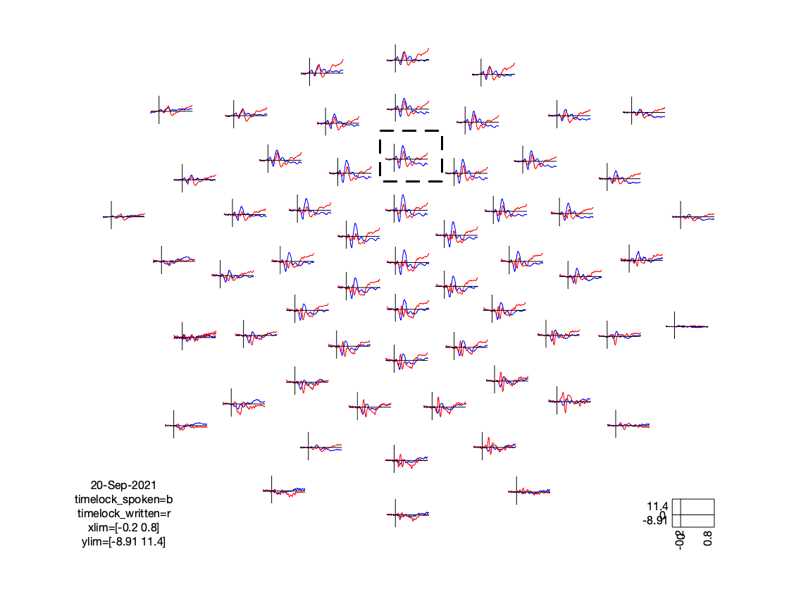
Visualize the individual conditions
cfg          = [];
cfg.layout   = 'dccn_customized_acticap64.mat';
cfg.colormap = {'*RdBu', 30};
ft_multiplotER(cfg, timelock_spoken, timelock_written);
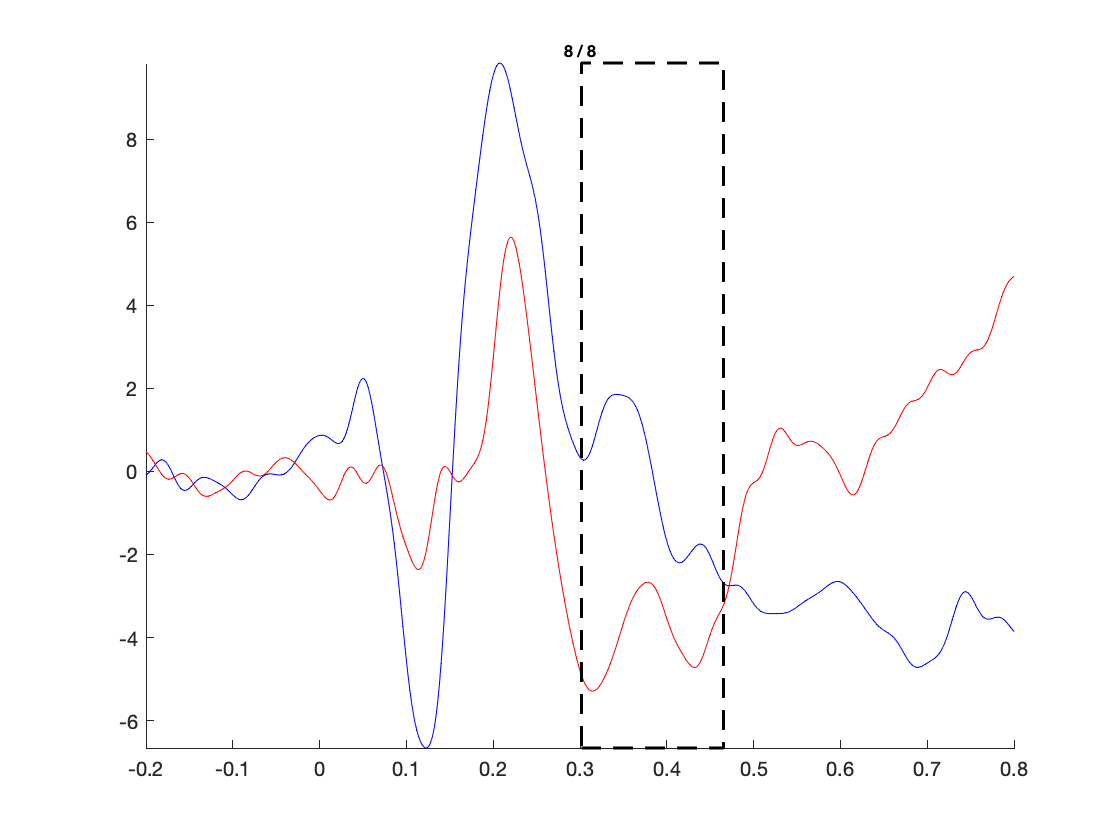
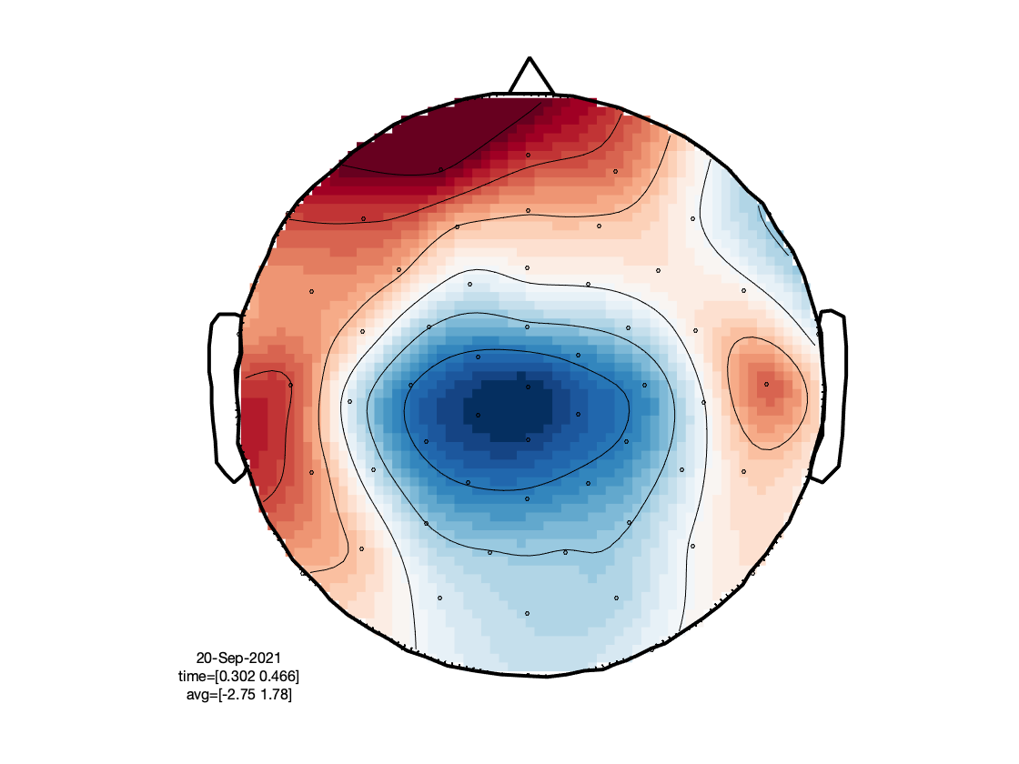
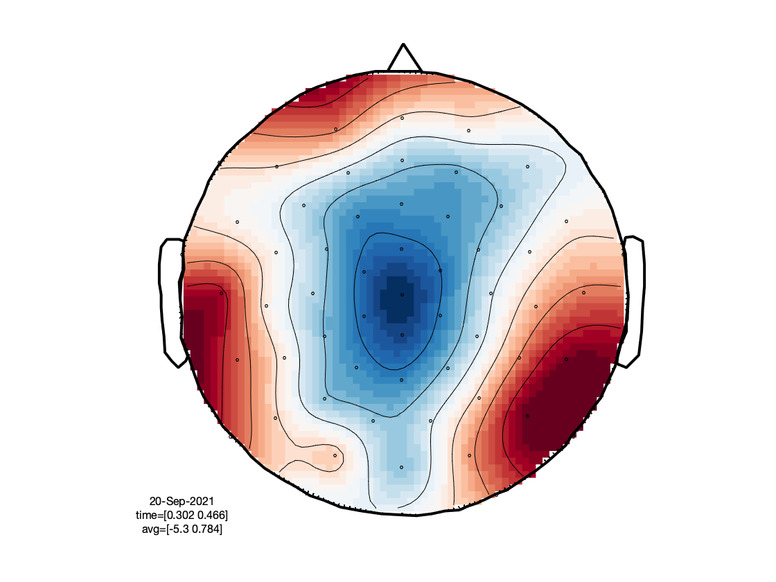
The figure that is generated by the above function call, is interactive, and it allows you to select (sets of) channels, and subsequently latency windows to investigate the spatial topography of event-related components:
Filter and average animals and tools category
Repeat the filtering and averaging, but now for a different partitioning of the epochs.
cfg                    = [];
cfg.preproc.lpfilter   = 'yes';
cfg.preproc.lpfreq     = 30;
cfg.preproc.lpfilttype = 'firws';

cfg.trials       = strcmp(data_segmented_clean.trialinfo.category, 'animals');
timelock_animals = ft_timelockanalysis(cfg, data_segmented_clean);

cfg.trials       = strcmp(data_segmented_clean.trialinfo.category, 'tools');
timelock_tools   = ft_timelockanalysis(cfg, data_segmented_clean);
Visualize the individual conditions
cfg          = [];
cfg.layout   = 'dccn_customized_acticap64.mat';
cfg.colormap = {'*RdBu', 30};
ft_multiplotER(cfg, timelock_animals, timelock_tools);
Compute differences: main effect of modality, main effect of category
cfg                  = [];
cfg.parameter        = 'avg';
cfg.operation        = 'x1-x2'; % subtract the 2nd from the 1st
animals_minus_tools  = ft_math(cfg, timelock_animals, timelock_tools);
spoken_minus_written = ft_math(cfg, timelock_spoken, timelock_written);
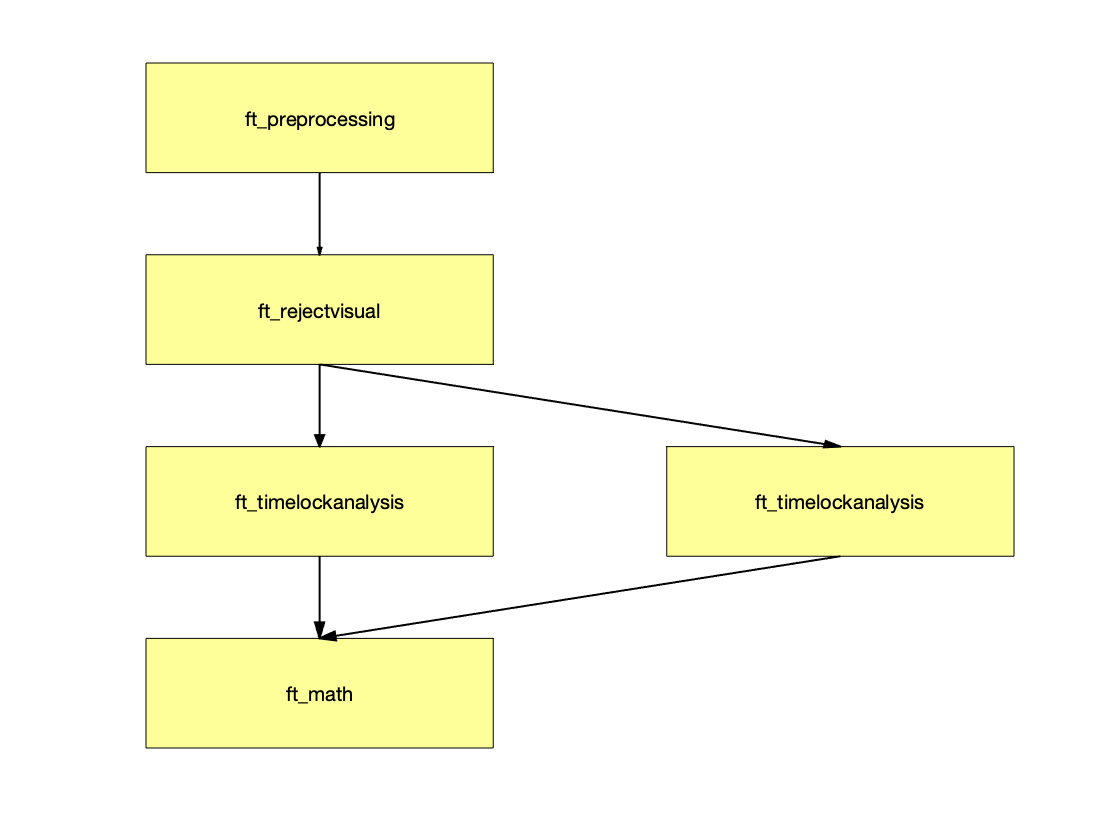
The ft_math function allows to perform mathematical operations on the numeric data, while keeping track of the processing steps. This is beneficial in relation to reproducibility of results. Specifically, the below could also easily be obtained by the creation of a new variable animals_minus_tools, and storing the difference in its ‘avg’ field: animals_minus_tools.avg = timelock_animals.avg - timelock_tools.avg. This is not ideal, since we could easily lose track of how the numeric data were actually generated. As an bonus exercise, you could explore the history of a FieldTrip variable by looking in its cfg field:
ft_analysispipeline([], spoken_minus_written);
which will show the following figure. You can click on the individual boxes to see the cfg details of the corresponding step.
Visualize the main effect of modality
cfg          = [];
cfg.layout   = 'dccn_customized_acticap64.mat';
cfg.colormap = {'*RdBu', 30};
ft_multiplotER(cfg, spoken_minus_written);
Epoching, TFRs, difference, visualization
Besides looking at the “evoked” effects that are captured in the event-related potentials, we can also look at “induced” effects, i.e. effects where the precise timing and/or phase of the effect vary over trials. This reqiures time-frequency analysis.
Define the epochs
The preprocessing here is very similar to that above, with the only difference that a longer time window is selected around each event, for the purpose of baseline correction (see below).
cfg         = [];
cfg.dataset = 'sub-02/eeg/sub-02_task-language_eeg.vhdr';
cfg.trialfun = 'ft_trialfun_bids';
cfg.trialdef.prestim  = 0.8;
cfg.trialdef.poststim = 1.2;
cfg.trialdef.task     = 'notarget';
cfg.trialdef.category = {'tools', 'animals'};

cfg = ft_definetrial(cfg);
As before, we will take this cfg with the added trl field to the next step of reading and preprocessing.
Load the data and rereference
cfg.demean         = 'yes';
cfg.baselinewindow = [-0.1 0];
cfg.reref          = 'yes';
cfg.channel        = {'all' '-61' '-62' '-63' '-64'};
cfg.implicitref    = 'M1';
cfg.refchannel     = {'M1', '53'};
data_segmented     = ft_preprocessing(cfg);
Reject artifacts
cfg         = [];
cfg.method  = 'summary';
cfg.layout  = 'dccn_customized_acticap64.mat';
data_segmented_clean = ft_rejectvisual(cfg, data_segmented);
Time-frequency analysis
The code below implements a wavelet-like analysis, i.e., it convolves the data with a sequence of Hanning-tapered basis functions (complex-valued sinusoids), the length of which scales with the frequency of interest. More information about the different methods to do time-frequency decomposition in FieldTrip can be found in another tutorial.
cfg = [];
cfg.method    = 'mtmconvol';
cfg.foi       = 1.25:1.25:40;
cfg.t_ftimwin = 4./cfg.foi;
cfg.taper     = 'hanning';
cfg.pad       = 4;
cfg.toi       = -0.5:0.02:0.9;

cfg.trials    = strcmp(data_segmented_clean.trialinfo.modality, 'written');
freq_written  = ft_freqanalysis(cfg, data_segmented_clean);

cfg.trials    = strcmp(data_segmented_clean.trialinfo.modality, 'spoken');
freq_spoken   = ft_freqanalysis(cfg, data_segmented_clean);
Compute the difference
Rather than plain subtracting, as we did with the ERP amplitudes, here we express the difference as the log-transformed difference. Since log(a)-log(b)=log(a/b), this difference is the same as the log-transformed ratio between the conditions.
cfg = [];
cfg.parameter = 'powspctrm';
cfg.operation = 'log10(x1)-log10(x2)';

spoken_minus_written = ft_math(cfg, freq_spoken, freq_written);
Baselining and visualization
Given the typical 1/f profile of spectra, i.e., low frequencies typically have orders of magnitude larger power than higher frequencies, it is custom to express the time varying (and frequency specific) power, relative to a baseline. Also, applying a baseline allows to investigate the extent to which power changes are induced by the experimental events. Note that - depending on the frequency of interest - the chosen baseline window below may lead to post-stimulus onset activity to ‘bleed’ into the baseline estimate.
cfg = [];
cfg.baseline = [-0.4 -0.2];
cfg.baselinetype = 'relchange';
freq_written = ft_freqbaseline(cfg, freq_written);
freq_spoken = ft_freqbaseline(cfg, freq_spoken);
cfg = [];
cfg.layout = 'dccn_customized_acticap64.mat';
cfg.zlim = 'maxabs';
cfg.colormap = {'*RdBu', 30};
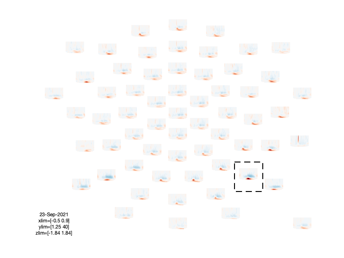
figure; ft_multiplotTFR(cfg, freq_written);
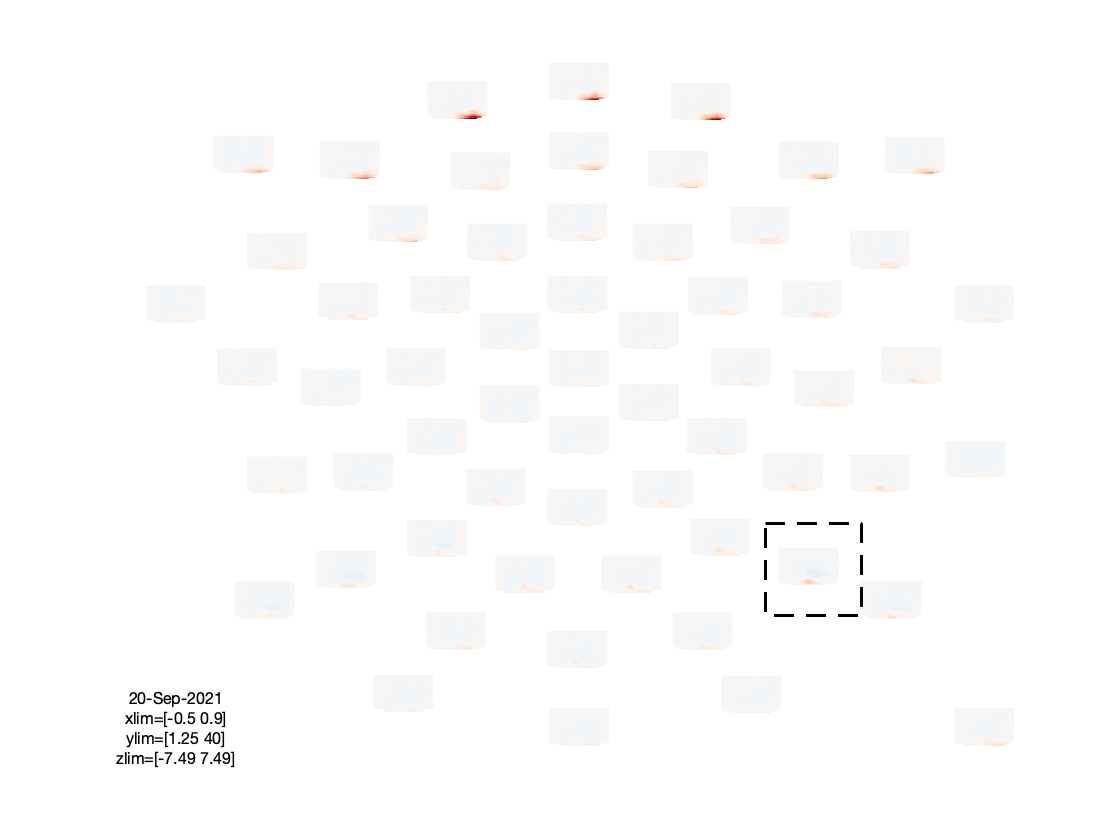
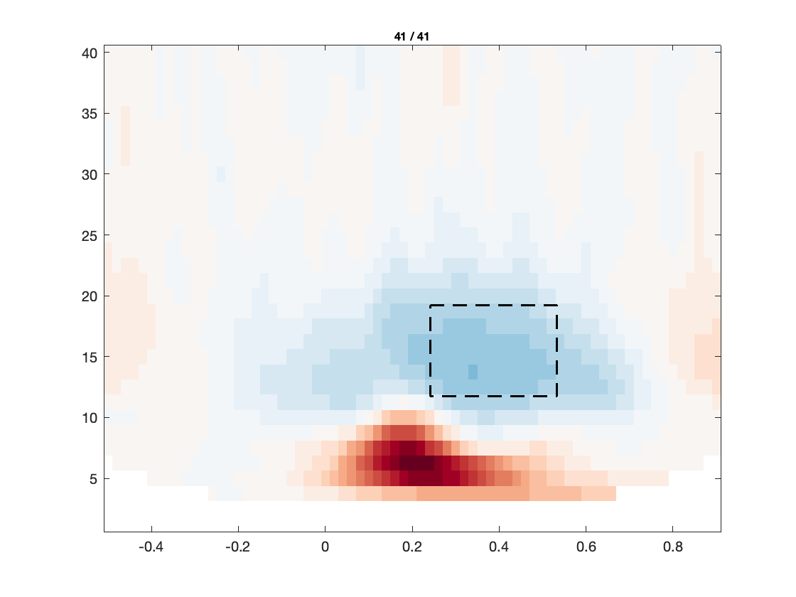
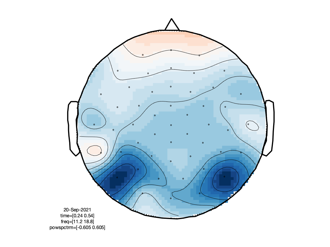
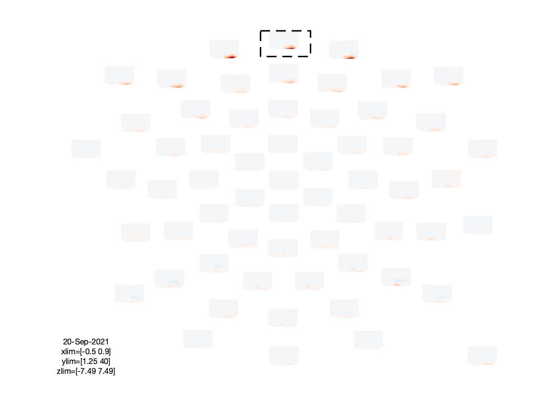
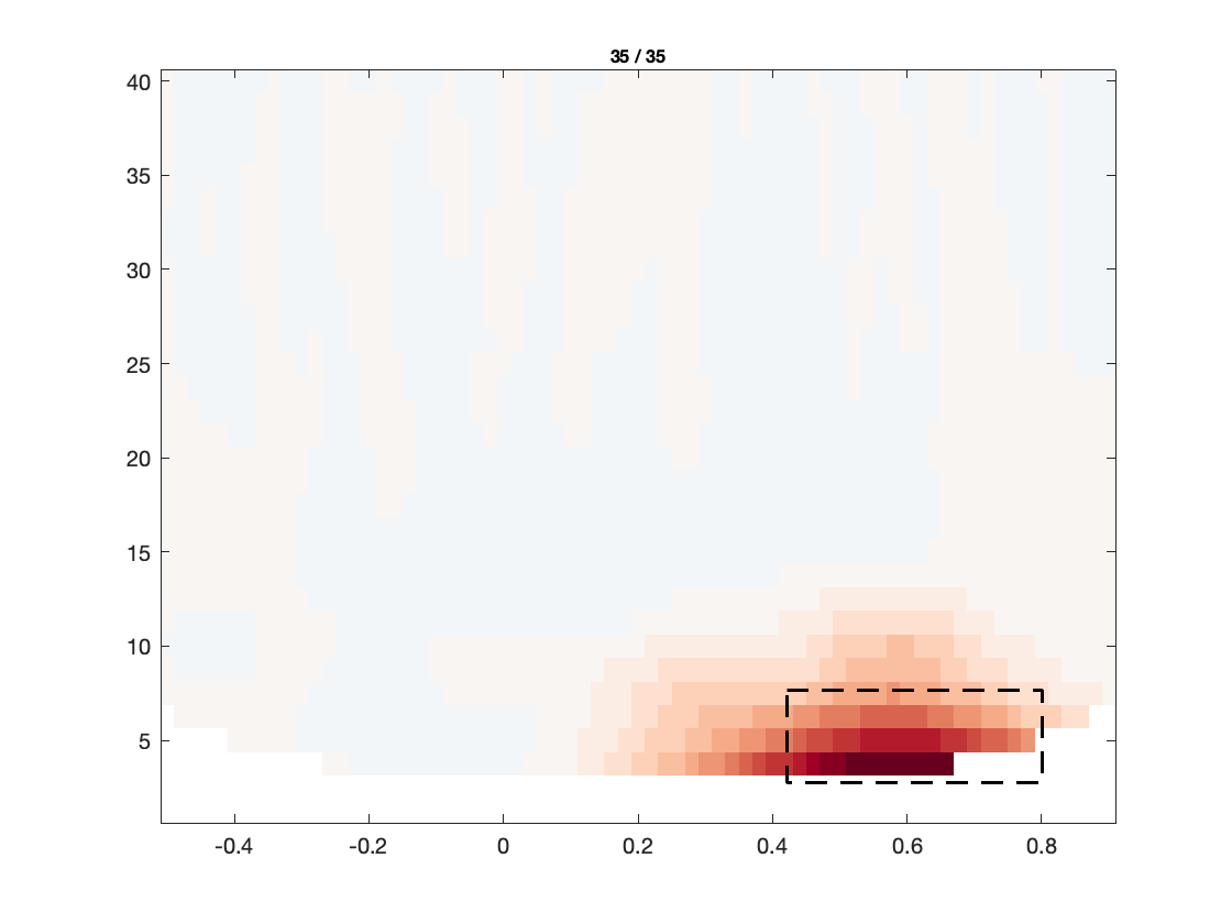
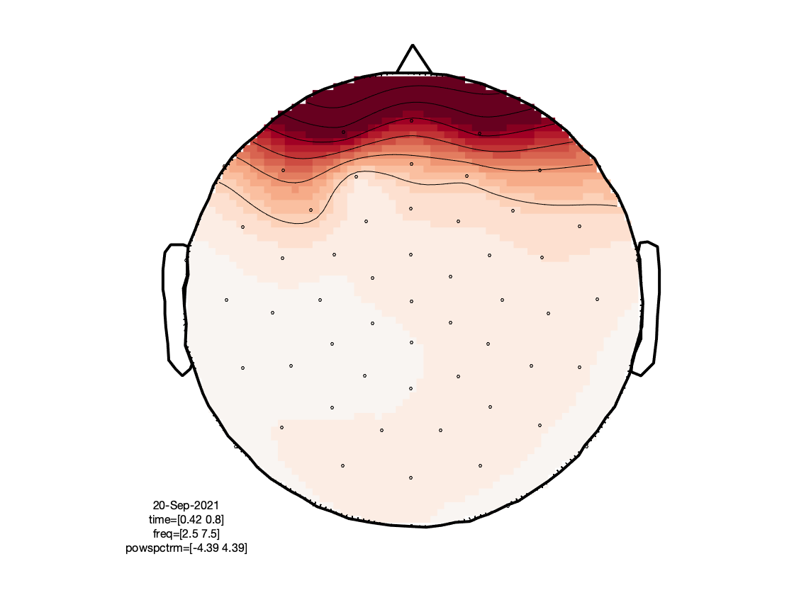
Based on the figures that we have produced, we can make a few observations:
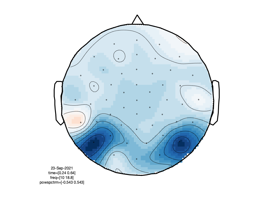
- There is an interesting event-related desynchronization (ERD) in the low-beta band, occurring between 0.2 and 0.5 seconds after stimulus onset.
- The spatial topography of the beta ERD has two focal minima in left posterior electrodes, and is thus suggestive of visual cortex activation.
- The TFRs of the frontal electrodes appear to be swamped by a large power low frequency effect.
Exercise: Explore the data of the other condition, as well as the difference between written and spoken presentation, by using the above chunk of code, but with the other variables in the input.
Excursion: EOG removal to reduce confounds
In this experiment we have both visual/written and auditory/spoken stimulus material. Although the ‘basic’ processing pipeline presented above allowed for interpretable TFRs, you were able to observe that eye movements and blinks contaminated the EEG data quite substantially. Particularly, when (involuntary) eye movements are not fully independent of the experimental manipulation (e.g., eye movements might occur more often in the written modality trials than in the spoken trials, or eye movements tend to occur after stimulus onset) these artifacts cause ‘structure’ in the data that does not reflect brain activity. For this reason it is common to ‘remove’ eye related signals from the data, for instance using independent component analysis or related techniques. Below, we use ‘DSS’, which is a nephew of ICA, to quickly identify and remove eye movement related signals.
Define the epochs
The trl array is used later.
cfg         = [];
cfg.dataset = 'sub-02/eeg/sub-02_task-language_eeg.vhdr';
cfg.trialfun = 'ft_trialfun_bids';
cfg.trialdef.prestim  = 0.8;
cfg.trialdef.poststim = 1.2;
cfg.trialdef.task     = 'notarget';
cfg.trialdef.category = {'tools', 'animals'};

cfg = ft_definetrial(cfg);
trl = cfg.trl;
Load in the data and rereference to linked mastoids, don’t epoch yet to facilitate the artifact handling
We want to use as much data as possible to identify the eye movement related activity, hence we do not epoch yet.
cfg             = [];
cfg.dataset     = 'sub-02/eeg/sub-02_task-language_eeg.vhdr';
cfg.reref       = 'yes';
cfg.channel     = {'all' '-61' '-62' '-63' '-64'};
cfg.implicitref = 'M1';             % the implicit (non-recorded) reference channel is added to the data
cfg.refchannel  = {'M1', '53'};     % the average of these will be the new reference, note that '53' corresponds to the right mastoid (M2)
data            = ft_preprocessing(cfg);
Extract the vEOG as separate data structure, to use for blink detection
Identify and remove eye blinks using the DSS algorithm. See this example for details.
cfg              = [];
cfg.dataset      = 'sub-02/eeg/sub-02_task-language_eeg.vhdr';
cfg.channel      = {'50' '64'};
cfg.reref        = 'yes';
cfg.implicitref  = []; % this is the default, we mention it here to be explicit
cfg.refchannel   = {'50'};
eogv             = ft_preprocessing(cfg);

cfg              = [];
cfg.channel      = '64';
eogv             = ft_selectdata(cfg, eogv);
eogv.label       = {'EOGv'};
The intention is to identify time points at which the blinks occurred, expressed as samples, relative to the onset of the recording. These time points will be identified automatically in the step below, by means of a thresholding procedure. However, the recording consisted of three blocks of trials, where the breaks in between ideally should be excluded from the artifact identification procedure (because the ‘dirt’ in the data is rather unspecific). To this end, we quickly identify the large outliers in the eog signal before proceeding. The three function calls below, temporarily cuts the continuous eog signal in smaller chunks, marks the ‘bad’ chunks as nans, and stitches them back together again into a continuous trace.
cfg            = [];
cfg.length     = 10;
eogv_segmented = ft_redefinetrial(cfg, eogv);

cfg            = [];
cfg.method     = 'summary';
cfg.keeptrial  = 'nan';
cfg.layout     = 'dccn_customized_acticap64.mat';
eogv_segmented_clean = ft_rejectvisual(cfg, eogv_segmented);

cfg            = [];
cfg.continuous ='yes';
eogv_stitched  = ft_redefinetrial(cfg, eogv_segmented_clean);
Peak detection of blinks
In this step, the approximate onsets of eye blinks are identified. This is based on a semi-automatic procedure, where the eog channel is bandpass filtered, rectified, z-scored, and thresholded.
cfg                                  = [];
cfg.artfctdef.zvalue.channel         = 'EOGv';
cfg.artfctdef.zvalue.cutoff          = 2
cfg.artfctdef.zvalue.interactive     = 'yes';
cfg.artfctdef.zvalue.bpfilter        = 'yes';
cfg.artfctdef.zvalue.bpfreq          = [1 20];
cfg.artfctdef.zvalue.bpfilttype      = 'firws';
cfg.artfctdef.zvalue.rectify         = 'yes';
cfg.artfctdef.zvalue.artfctpeak      = 'yes';
cfg.artfctdef.zvalue.artfctpeakrange = [-.25 .5]; % save out 250ms prior and 500ms post ECG peak
cfg = ft_artifact_zvalue(cfg, eogv_stitched);
Estimate components wit the denoising source separation (DSS) algorithm
DSS is a blind source separation algorithm that aims at identifying underlying sources based on some constraints. Here, the sources are separated based on the constraint that they show a large signal time-locked to the eye blink (hence the peak detection in the previous step).
% specify the DSS parameters for ft_componentanalysis
params.artifact = cfg.artfctdef.zvalue.artifact;
params.demean = true;

cfg                   = [];
cfg.method            = 'dss';
cfg.dss.denf.function = 'denoise_avg2';
cfg.dss.denf.params   = params;
cfg.numcomponent      = 5;
cfg.cellmode          = 'yes';
comp                  = ft_componentanalysis(cfg, data);

cfg           = [];
cfg.layout    = 'dccn_customized_acticap64.mat';
cfg.eogscale  = 10;
cfg.ylim      = [-1500 1500];
cfg.blocksize = 10;
ft_databrowser(cfg, ft_appenddata([], eogv, comp));
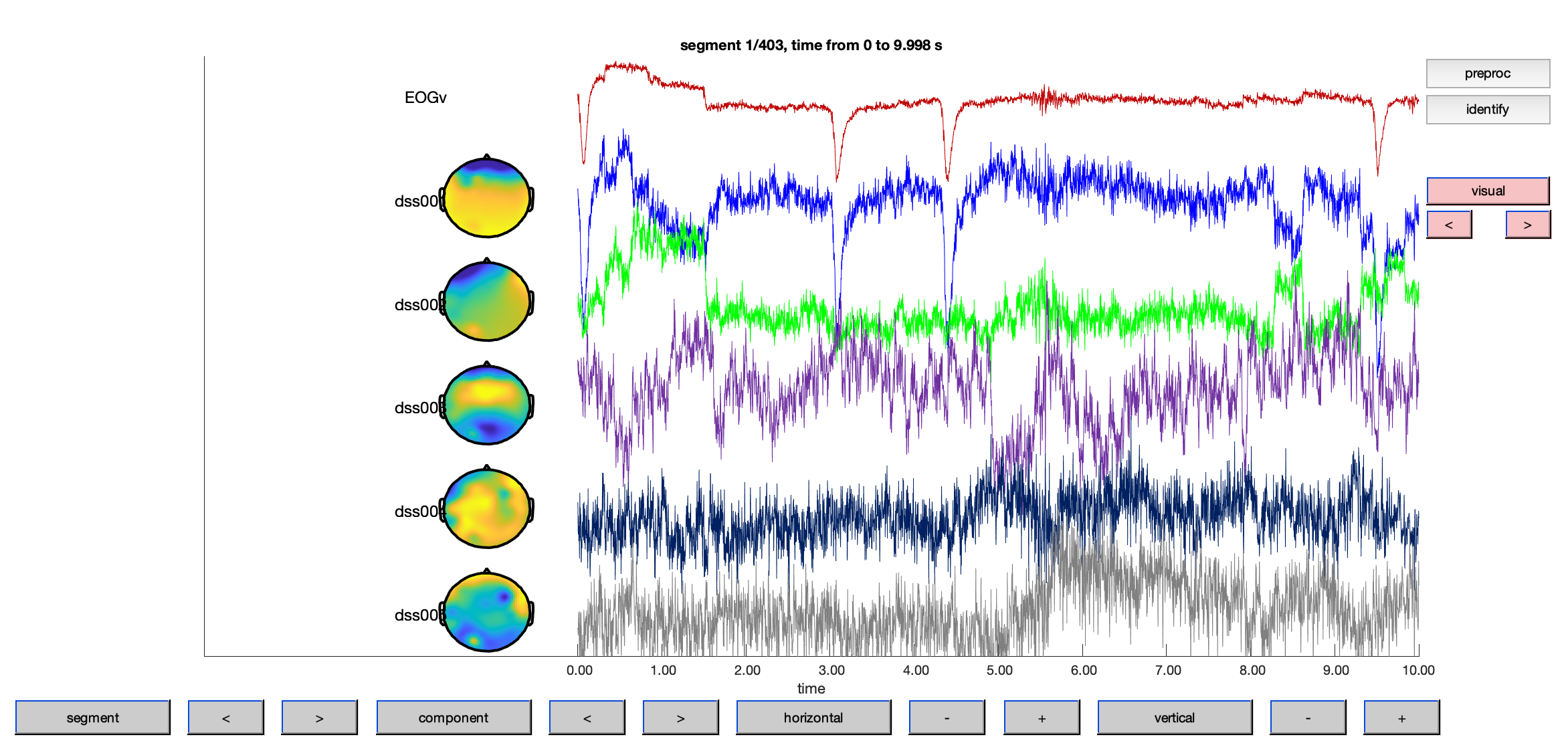
Judging from the topographies and the time courses of the components, components 1 and 2 are identified as eye-related, so they are removed in the next step.
cfg           = [];
cfg.component = [1 2];
cfg.layout    = 'dccn_customized_acticap64.mat';
data_dss      = ft_rejectcomponent(cfg, comp, data);
Epoch the data
Proceed with the rest of the analysis, but now on the cleaned data. This is mostly the same as how it was done above.
cfg     = [];
cfg.trl = trl;
data_dss_segmented = ft_redefinetrial(cfg, data_dss);
Reject trials and/or channels with other artifacts
cfg         = [];
cfg.method  = 'summary';
cfg.layout  = 'dccn_customized_acticap64.mat';
data_dss_segmented_clean = ft_rejectvisual(cfg, data_dss_segmented);
Time-frequency analysis
cfg = [];
cfg.method    = 'mtmconvol';
cfg.foi       = 1.25:1.25:40;
cfg.t_ftimwin = 4./cfg.foi; % 0.8.*ones(size(cfg.foi));
cfg.taper     = 'hanning';
cfg.pad       = 4;
cfg.toi       = -0.5:0.02:0.9;

cfg.trials      = strcmp(data_dss_segmented_clean.trialinfo.modality, 'written');
freqdss_written = ft_freqanalysis(cfg, data_dss_segmented_clean);

cfg.trials      = strcmp(data_dss_segmented_clean.trialinfo.modality, 'spoken');
freqdss_spoken  = ft_freqanalysis(cfg, data_dss_segmented_clean);
Compute the difference
cfg = [];
cfg.parameter = 'powspctrm';
cfg.operation = 'log10(x1)-log10(x2)';

spoken_minus_written_dss = ft_math(cfg, freqdss_spoken, freqdss_written);
Baselining and visualization
cfg = [];
cfg.baseline = [-0.4 -0.2];
cfg.baselinetype = 'relchange';
freqdss_written = ft_freqbaseline(cfg, freqdss_written);
freqdss_spoken  = ft_freqbaseline(cfg, freqdss_spoken);

cfg          = [];
cfg.layout   = 'dccn_customized_acticap64.mat';
cfg.zlim     = 'maxabs';
cfg.colormap = {'*RdBu', 30};
figure; ft_multiplotTFR(cfg, freqdss_written);

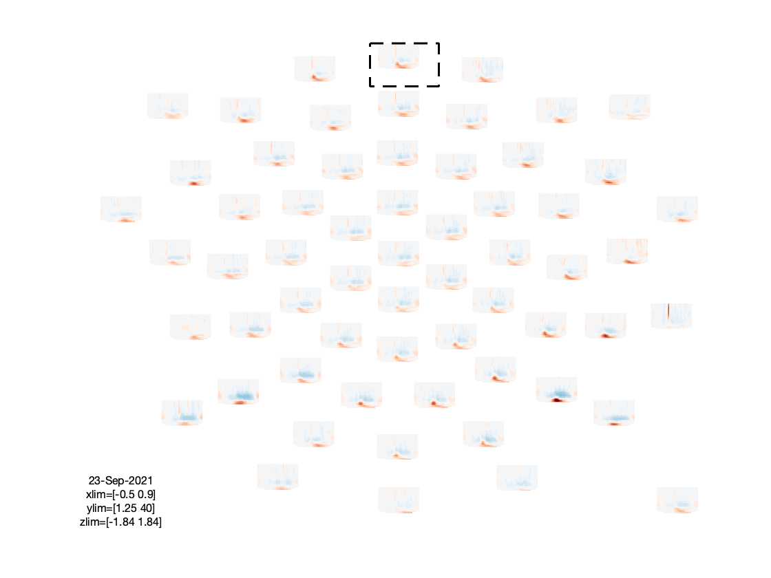
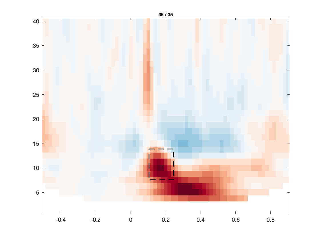
The figures investigate the same individual channels’ TFRs, and the corresponding topographies of prominent features therein. As can be seen, the effect of the eye blink removal has hardly an effect on the TFR in the right occipital electrode, but makes a big difference for the frontal electrode. Even though there still seems to be a residual of the eye blinks in the TFR after DSS, the TFR now reveals more clearly an occipital increase in power between 8 and 15 Hz, around 100-200 ms after stimulus onset. This is most likely the frequency transform of the stimulus-evoked transient, and does not necessarily reflect an oscillation in the alpha band/low beta band.
Exercise: Explore the data of the other condition, as well as the difference between written and spoken presentation, by using the above chunk of code, but with the other variables in the input. Inspect how these figures compare to the same data, but without the DSS eye blink removal applied.
Continuous analysis, chunked spectral decomposition
And now for something completely different. The next part of this tutorial deals with an analysis that treats the data more as a continuous chunk, rather than a collection of experimentally relevant epochs. The idea behind this, is that there might be fluctuations in some aspects of the brain signals, on longer time scales than the relevant cognitive events, which could interact with the way in which the brain responds to those events. Below we are going to perform a time-frequency analysis on the whole >1 hour recording. This part of the tutorial can be explored on itself, for which the data needs to be processed from the raw datafile.
Load the continuous data or use the cleaned continuous data computed earlier
If you did not perform the previous parts of the tutorial, you should start from scratch:
cfg             = [];
cfg.dataset     = 'sub-02/eeg/sub-02_task-language_eeg.vhdr';
cfg.reref       = 'yes';
cfg.channel     = {'all' '-61' '-62' '-63' '-64'};
cfg.implicitref = 'M1';             % the implicit (non-recorded) reference channel is added to the data
cfg.refchannel  = {'M1', '53'};     % the average of these will be the new reference, note that '53' corresponds to the right mastoid (M2)
data            = ft_preprocessing(cfg);
Alternatively, if you have performed the previous parts of the tutorial, you could start from using the continuous data that has been cleaned from eye blink related artifacts. We used those data for the figures presented below.
data = data_dss;
Segment the continuous data in overlapping chunks
Although the data will now be segmented, the consecutive individual ‘epochs’ still represent a continuous sequence of intermediate length pieces of data (in the below case) of 5 seconds long. These pieces of data can for instance be used to estimate slow fluctuations in power at specific frequencies, on a slower time scale than the individual trials. Still, such an analysis might provide relevant information, because it could reveal fluctuations in alpha power that might serve as a proxy for fluctuations in arousal or engagement with the task. Such estimates could then subsequently be used as a confound for more sophisticated statistical modelling of experimental effects in the data. For instance, rather than computing experimental effects based on difference in the mean one could consider using a generalized linear model (GLM).
After cutting the continuous data into artificial epochs for spectral analysis, we will stitch the data back together again. As a side note, you may rightfully ask why this is done, since we could just as well compute a Time-frequency representation of the continuous data right away? The answer is that this conceptually is indeed what one wants to achieve, yet it’s computationally not feasible. Here, we are dealing with a more than one hour long recording, consisting of more than 2.000.000 samples. Imagine what would happen with a night long sleep recording!
cfg = [];
cfg.length  = 5;
cfg.overlap = 0.5; % between 0 and 1
data_segmented = ft_redefinetrial(cfg, data);
Identify and replace artifacts with NaNs
cfg = [];
cfg.keepchannel = 'yes';
cfg.keeptrial   = 'nan';
cfg.layout      = 'dccn_customized_acticap64.mat';
data_segmented_clean = ft_rejectvisual(cfg, data_segmented);
Compute power spectra
ft_warning off FieldTrip:dataContainsNaN

cfg = [];
cfg.method     = 'mtmfft';
cfg.taper      = 'dpss';
cfg.tapsmofrq  = 0.5;
cfg.keeptrials = 'yes';
freq_segmented = ft_freqanalysis(cfg, data_segmented_clean);
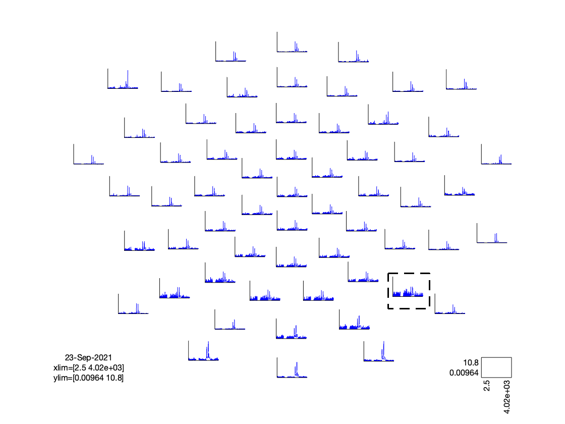
Average across the pseudo-epochs
cfg = [];
cfg.avgoverrpt = 'yes';
cfg.keeprptdim = 'no';
%cfg.trials = ~isnan(freq_segmented.powspctrm(:,1,1));
cfg.nanmean = 'yes';
freq_spectrum = ft_selectdata(cfg, freq_segmented);
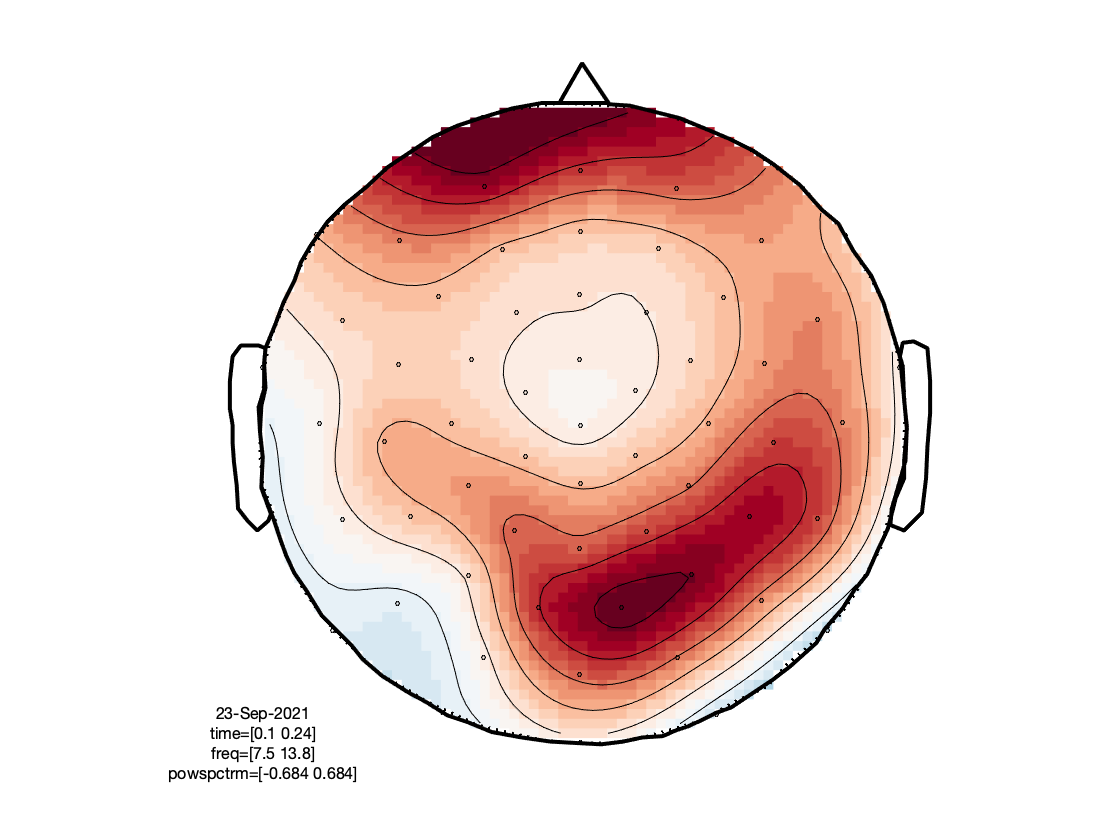
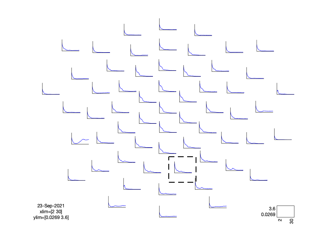
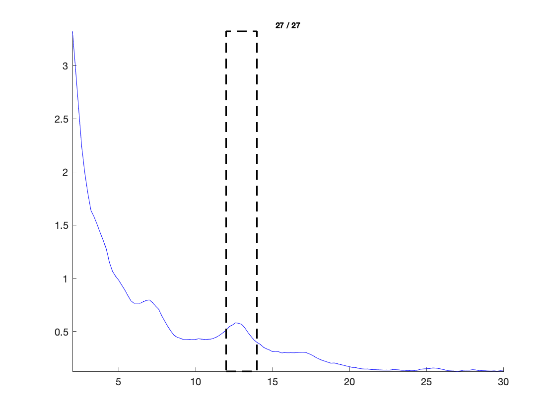
cfg = [];
cfg.layout = 'dccn_customized_acticap64.mat';
cfg.parameter = 'powspctrm';
cfg.xlim = [2 30];
cfg.colormap = {'*RdBu', 30};
ft_multiplotER(cfg, freq_spectrum);
Reorganize the data
Now we do a little bit of data voodoo (outside FieldTrip), in order to reorganize the data back onto the original time axis of the recording.
begsample = data_segmented.sampleinfo(:,1);
endsample = data_segmented.sampleinfo(:,2);
time = ((begsample+endsample)/2) / data_segmented.fsample;

freq_continuous           = freq_segmented;
freq_continuous.powspctrm = permute(freq_segmented.powspctrm, [2, 3, 1]);
freq_continuous.dimord    = 'chan_freq_time'; % it used to be 'rpt_chan_freq'
freq_continuous.time      = time;             % add the description of the time dimension
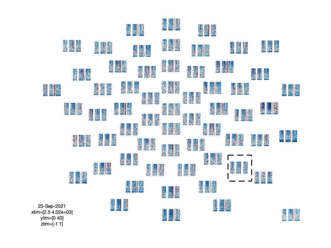
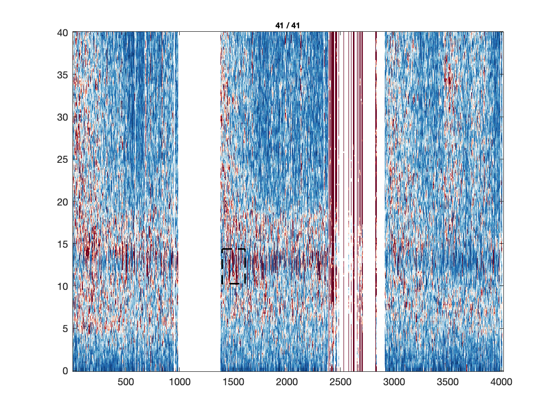
Visualization
Note that here the plotting function takes care of the baselining under the hood.
cfg = [];
cfg.layout   = 'dccn_customized_acticap64.mat';
cfg.baseline = [-inf inf];
cfg.baselinetype = 'relchange';
cfg.ylim     = [0 40];
cfg.zlim     = [-1 1];
cfg.colormap = {'*RdBu', 30};
ft_multiplotTFR(cfg, freq_continuous);
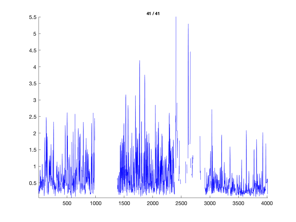
Extract the almost alpha band power
cfg = [];
cfg.frequency   = [12 14];
cfg.avgoverfreq = 'yes';
cfg.keepfreqdim = 'no';
timelock_alpha  = ft_selectdata(cfg, freq_continuous);
Reorganize from freq to timelock structure
timelock_alpha.avg = timelock_alpha.powspctrm;
timelock_alpha = rmfield(timelock_alpha, 'cumsumcnt');
timelock_alpha = rmfield(timelock_alpha, 'cumtapcnt');
timelock_alpha = rmfield(timelock_alpha, 'powspctrm');
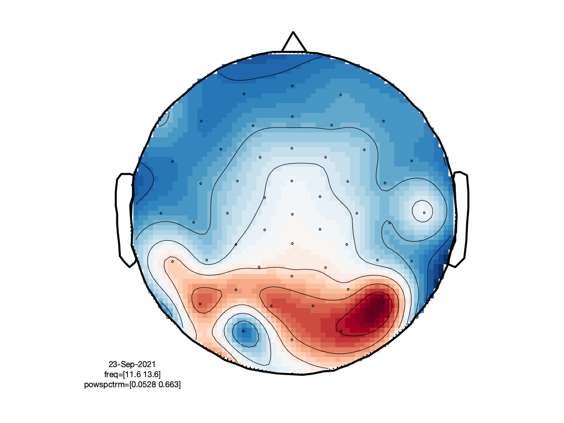
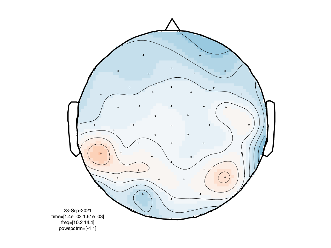
Visualize the result
cfg          = [];
cfg.layout   = 'dccn_customized_acticap64.mat';
cfg.colormap = {'*RdBu', 30};
ft_multiplotER(cfg, timelock_alpha);
Summary and conclusion
In this tutorial we demonstrated EEG preprocessing, event-related potentials (ERPs), artifact removal using DSS, time-frequency analysis and continuous analysis.
The next steps in the analysis that are not covered here would consist of processing the data from more participants and doing statistics. You could continue with one of the following:
- Creating a clean and efficient analysis script
- You can follow one of the tutorials on statistics
- You can look at the example scripts for GLM on time series data or GLM over trials
- You can have a look at the sleep tutorial to learn more about the analysis of long continuous recordings