FieldTrip beamformer demo

%% get data from SPM

D = spm_eeg_load('../spm-source-demo/PapMcbdspmeeg_run_01_sss.mat');

% convert sensors and volume conduction model from SPM
volsens = spm_eeg_inv_get_vol_sens(D, 1, 'Head', 'inv', 'MEG');
vol1    = volsens.MEG.vol;
sens1   = volsens.MEG.sens;
mri1    = ft_read_mri('../spm-source-demo/mprage.nii');

%% start from scratch data in FieldTrip

subj = 15;
prefix = sprintf('Sub%02d', subj);
load([prefix '_raw']);  % this is called "data" rather than "raw"

sens = data.grad;

% load the original MRI
mri_orig = ft_read_mri('../data/Sub15/T1/mprage.nii');

% load the positions of the anatomical fiducials (as provided by Rik)
load('../data/Sub15/T1/mri_fids.mat');

headshape = ft_read_headshape('../data/Sub15/MEEG/run_01_raw.fif');
headshape = ft_convert_units(headshape, 'mm');

% the MRI is neither expressed in MNI, nor in Neuromag coordinates
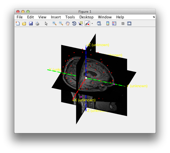
ft_determine_coordsys(mri_orig, 'interactive', 'no');
hold on; % add the subsequent objects to the same figure
ft_plot_headshape(headshape);
plot3(mri_fids(1,1), mri_fids(1,2), mri_fids(1,3), 'm*');
plot3(mri_fids(2,1), mri_fids(2,2), mri_fids(2,3), 'm*');
plot3(mri_fids(3,1), mri_fids(3,2), mri_fids(3,3), 'm*');

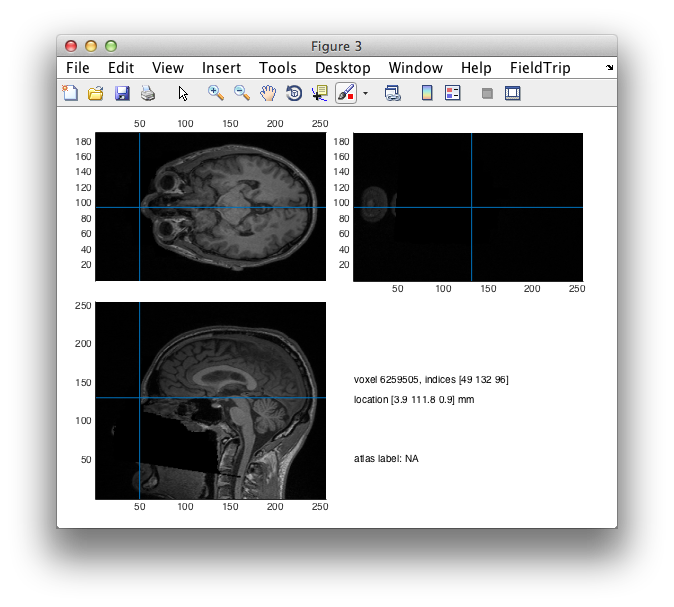
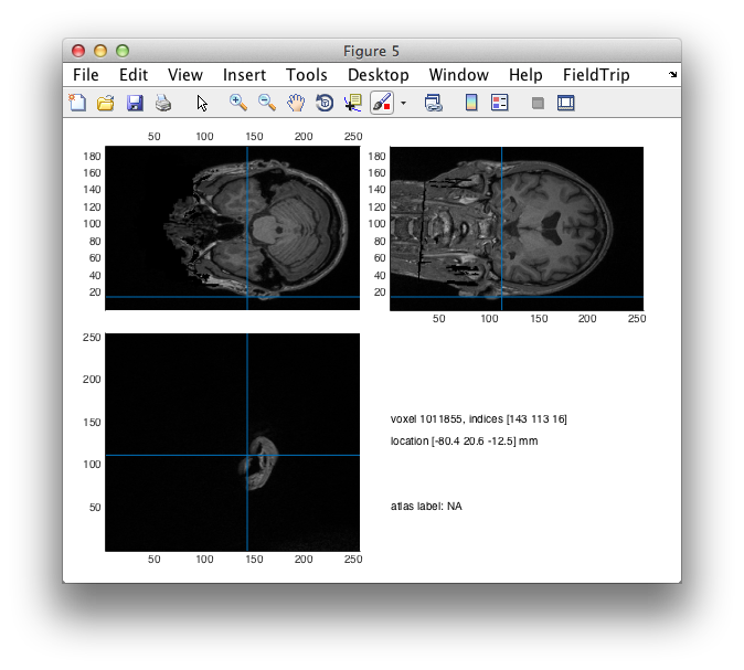
%% validate the positions of the fiducials that were provided by Rik

cfg = [];
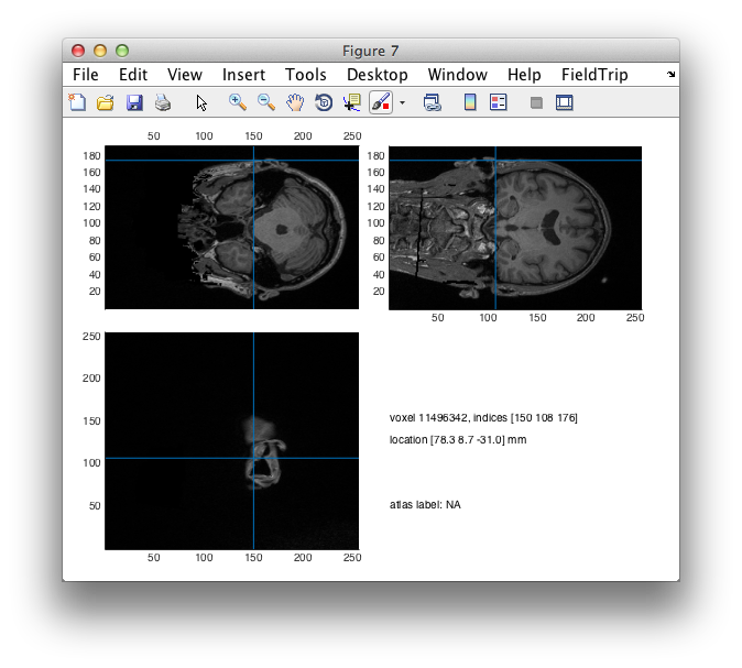
cfg.location = mri_fids(1,:);
ft_sourceplot(cfg, mri_orig);

cfg = [];
cfg.location = mri_fids(2,:);
ft_sourceplot(cfg, mri_orig);

cfg = [];
cfg.location = mri_fids(3,:);
ft_sourceplot(cfg, mri_orig);

%%

% the location of fiducials is expressed in original MRI coordinates
% ft_volumerealign needs them in voxel coordinates
vox_fids = ft_warp_apply(inv(mri_orig.transform), mri_fids);

cfg = [];
cfg.fiducial.nas = vox_fids(1,:);
cfg.fiducial.lpa = vox_fids(2,:);
cfg.fiducial.rpa = vox_fids(3,:);
cfg.coordsys = 'neuromag';
mri_realigned = ft_volumerealign(cfg, mri_orig);

% save mri_realigned mri_realigned

% check that the MRI is consistent after realignment
ft_determine_coordsys(mri_realigned, 'interactive', 'no');
hold on; % add the subsequent objects to the figure
drawnow; % workaround to prevent some MATLAB versions (2012b and 2014b) from crashing
ft_plot_headshape(headshape);

%%

cfg = [];
cfg.output = {'brain' 'scalp' 'skull'};
seg = ft_volumesegment(cfg, mri_realigned);

% save seg seg

%%

cfg = [];
cfg.method = 'projectmesh';
cfg.numvertices = 2000;
cfg.tissue = 'brain';
brain = ft_prepare_mesh(cfg, seg);
cfg.tissue = 'skull';
skull = ft_prepare_mesh(cfg, seg);
cfg.tissue = 'scalp';
scalp = ft_prepare_mesh(cfg, seg);

% save brain brain
% save skull skull
% save scalp scalp

%% make the volume conduction model

cfg = [];
cfg.method = 'singleshell';
vol = ft_prepare_headmodel(cfg, brain);

% save vol vol
% save sens sens

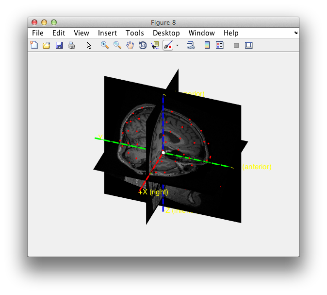
ft_determine_coordsys(mri_realigned, 'interactive', 'no')
hold on; % add the subsequent objects to the same figure
ft_plot_headshape(headshape);
ft_plot_headmodel(ft_convert_units(vol, 'mm'));

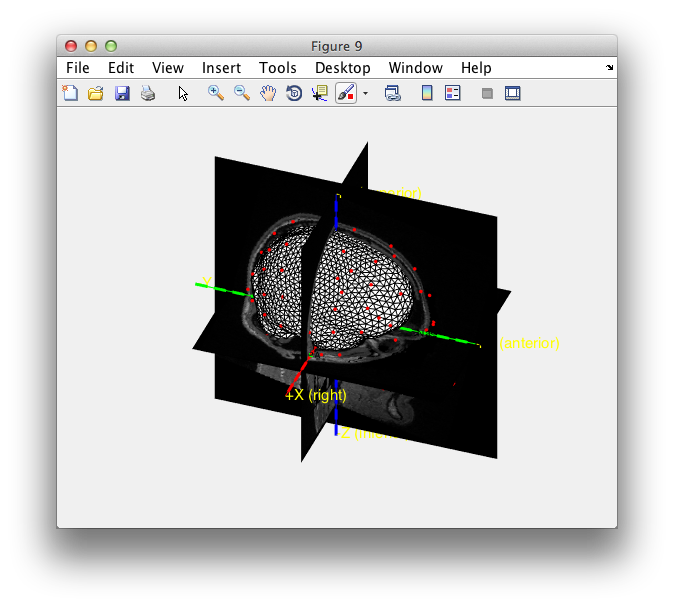
figure
hold on; % add the subsequent objects to the same figure
ft_plot_headshape(headshape);
ft_plot_sens(ft_convert_units(sens, 'mm'), 'coil', 'yes', 'coilsize', 10);
ft_plot_headmodel(ft_convert_units(vol, 'mm'));

figure
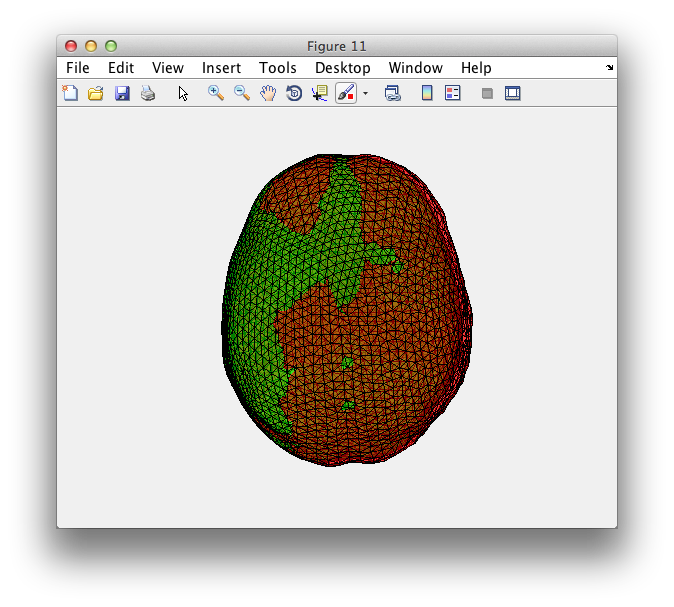
ft_plot_headmodel(ft_convert_units(vol,  'mm'), 'facecolor', 'r'); % FT
ft_plot_headmodel(ft_convert_units(vol1, 'mm'), 'facecolor', 'g'); % SPM
alpha 0.5

%% get data from SPM

D = spm_eeg_load('../spm-source-demo/PapMcbdspmeeg_run_01_sss.mat');

disp(D.condlist)

% convert data from SPM
raw      = D.ftraw(D.indchantype('MEGMAG'), D.indsample(-0.1):D.indsample(0.3), D.indtrial(D.condlist{1}, 'GOOD'));
timelock = D.fttimelock(D.indchantype('MEGMAG'), D.indsample(-0.1):D.indsample(0.3), D.indtrial(D.condlist{1}, 'GOOD'));

% alternative method
raw      = spm2fieldtrip(D);
timelock = ft_timelockanalysis([], raw);


%% start from data that was processed by FieldTrip
subj = 15;
prefix = sprintf('Sub%02d', subj);
load([prefix '_raw']);  % this is called "data" rather than "raw"
load([prefix '_avg_Faces_vs_Scrambled']);
load([prefix '_avg_Famous']);
load([prefix '_avg_Unfamiliar']);
load([prefix '_avg_Scrambled']);

% load the results from part 1
load vol
load sens


%% deal with maxfilter

% the data has been maxfiltered and subsequently contatenated
% this results in an ill-conditioned estimate of covariance or CSD

cfg = [];
cfg.method = 'pca';
cfg.updatesens = 'no';
cfg.channel = 'MEGMAG';
comp = ft_componentanalysis(cfg, data);

cfg = [];
cfg.updatesens = 'no';
cfg.component = comp.label(51:end);
data_fix = ft_rejectcomponent(cfg, comp);


%%

cfg = [];
cfg.channel = 'MEGMAG';
cfg.method = 'wavelet';
cfg.output = 'powandcsd';
cfg.foi = 4:2:70;
cfg.toi = -0.200:0.020:1.000;
wavelet = ft_freqanalysis(cfg, data_fix);

% save wavelet wavelet

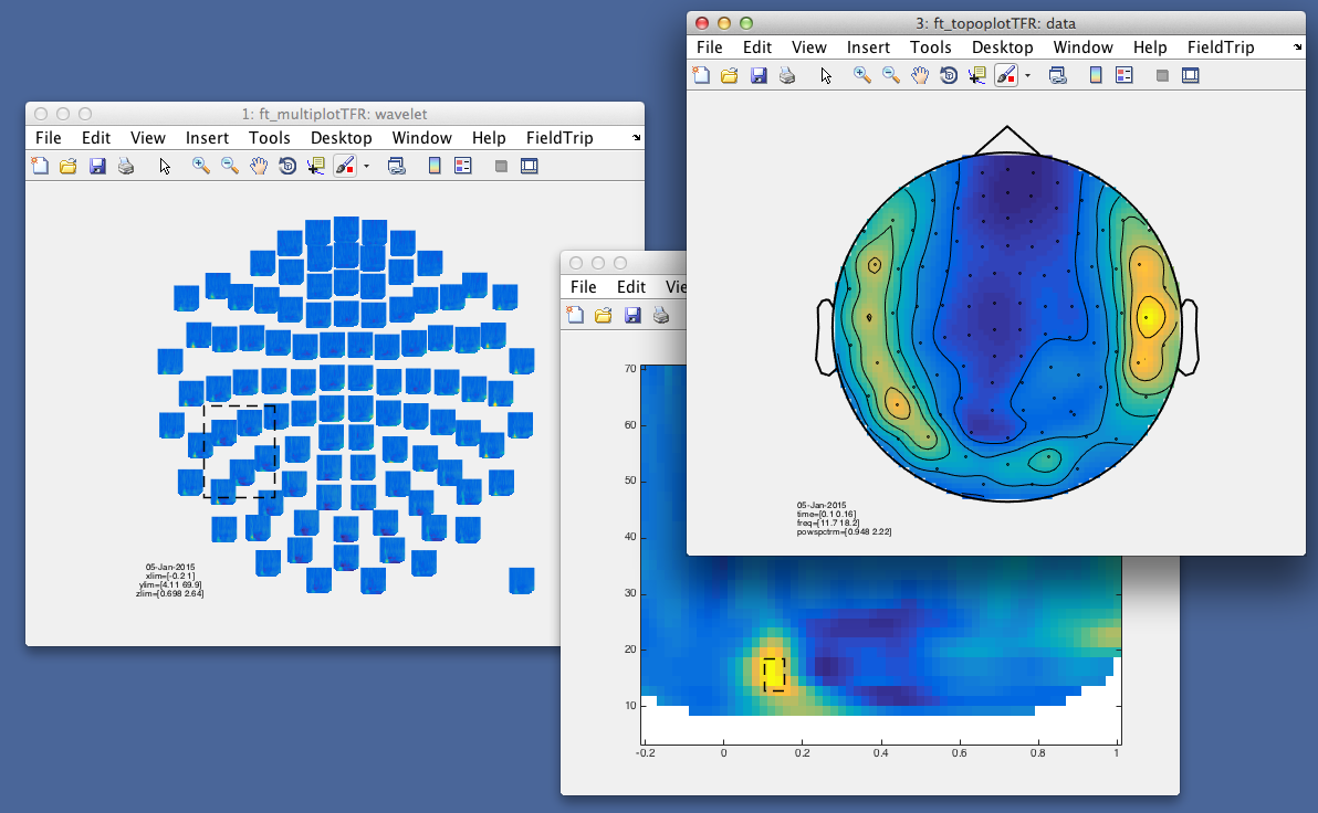
cfg = [];
cfg.layout = 'neuromag306mag.lay';
cfg.baseline = [-inf 0];
cfg.baselinetype = 'relative';
ft_multiplotTFR(cfg, wavelet)

%%

cfg = [];
cfg.resolution = 7;
% cfg.inwardshift = -7; % allow dipoles 10mm outside the brain, this improves interpolation at the edges
cfg.unit = 'mm';
cfg.headmodel = vol;  % from FT
cfg.grad = sens; % from FT
cfg.senstype = 'meg';
cfg.normalize = 'yes';
grid = ft_prepare_leadfield(cfg, wavelet);

% save grid grid


%% perform whole-brain source reconstruction

cfg = [];
cfg.headmodel = vol;  % from FT
cfg.grad      = sens; % from FT
cfg.senstype  = 'meg';
cfg.grid      = grid;
cfg.method    = 'dics';

cfg.frequency = [14 18];
cfg.latency   = [0.140 0.160];
sourceA = ft_sourceanalysis(cfg, wavelet);
cfg.latency   = [-0.100 -0.080];
sourceB = ft_sourceanalysis(cfg, wavelet);

% cfg.frequency = [40 65];
% cfg.latency   = [0.090 0.140];
% sourceA = ft_sourceanalysis(cfg, wavelet);
% cfg.latency   = [-0.100 -0.050];
% sourceB = ft_sourceanalysis(cfg, wavelet);

%
% cfg.frequency = [12 20];
% cfg.latency   = [0.090 0.140];
% sourceA = ft_sourceanalysis(cfg, wavelet);
% cfg.latency   = [-0.050 0.000];
% sourceB = ft_sourceanalysis(cfg, wavelet);

% FT_MATH requires the time axis needs to be the same
sourceA.time = 0;
sourceB.time = 0;

cfg = [];
cfg.parameter = 'pow';
cfg.operation = 'log10(x1/x2)'; % sourceA divided by sourceB
sourceR = ft_math(cfg, sourceA, sourceB);

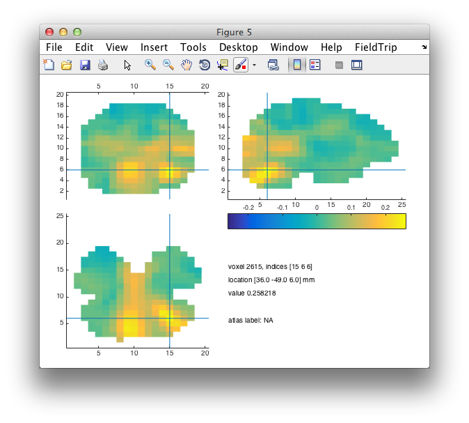
cfg = [];
cfg.funparameter = 'pow';
ft_sourceplot(cfg, sourceR);

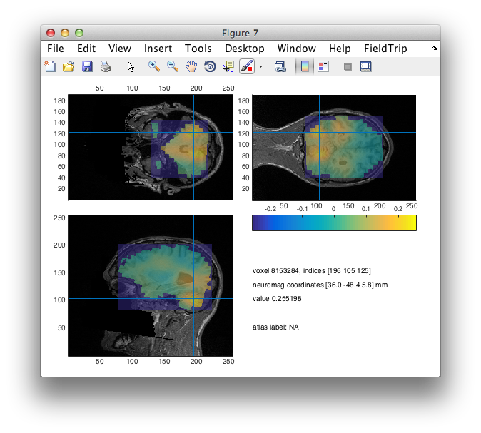
%% interpolate and plot on individual anatomical MRI

cfg = [];
cfg.parameter = 'pow';
sourceI = ft_sourceinterpolate(cfg, sourceR, mri_realigned);

cfg = [];
cfg.funparameter = 'pow';
ft_sourceplot(cfg, sourceI);

%% start from data that was processed by FieldTrip
subj = 15;
prefix = sprintf('Sub%02d', subj);
load([prefix '_raw']);  % this is called "data" rather than "raw"

%% deal with maxfilter

% the data has been maxfiltered and subsequently concatenated
% this results in an ill-conditioned estimate of covariance or CSD

cfg = [];
cfg.method = 'pca';
cfg.updatesens = 'no';
cfg.channel = 'MEGMAG';
comp = ft_componentanalysis(cfg, data);

cfg = [];
cfg.updatesens = 'no';
cfg.component = comp.label(51:end);
data_fix = ft_rejectcomponent(cfg, comp);

%% compute covariance

cfg = [];
cfg.channel = 'MEGMAG';
cfg.covariance = 'yes'; % compute the covariance for single trials, then average
% cfg.preproc.bpfilter = 'yes';
% cfg.preproc.bpfreq = [5 70];
% cfg.preproc.hpfilter = 'yes';
% cfg.preproc.hpfreq = 1;
% cfg.preproc.derivative = 'yes';
cfg.preproc.demean = 'yes';             % the PCA cleanup shifted the baseline
cfg.preproc.baselinewindow = [-inf 0];  % reapply the baseline correction
cfg.keeptrials = 'yes';
timelock1 = ft_timelockanalysis(cfg, data_fix);

cfg = [];
cfg.covariance = 'yes'; % compute the covariance of the averaged ERF
timelock2 = ft_timelockanalysis(cfg, timelock1);

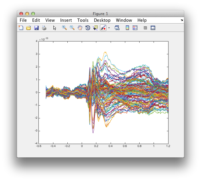
figure
plot(timelock2.time, timelock2.avg)

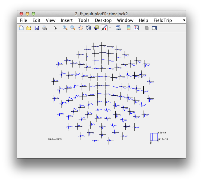
cfg = [];
cfg.layout = 'neuromag306mag.lay';
figure; ft_multiplotER(cfg, timelock2);

%%

pos = [21 -64 30];

cfg = [];
cfg.sourcemodel.pos = pos;
cfg.unit = 'mm';
% cfg.grid = grid;
cfg.headmodel = vol;
cfg.grad = sens;
cfg.senstype = 'meg';
cfg.method = 'lcmv';
cfg.lcmv.keepfilter = 'yes';
cfg.lcmv.projectmom = 'yes';
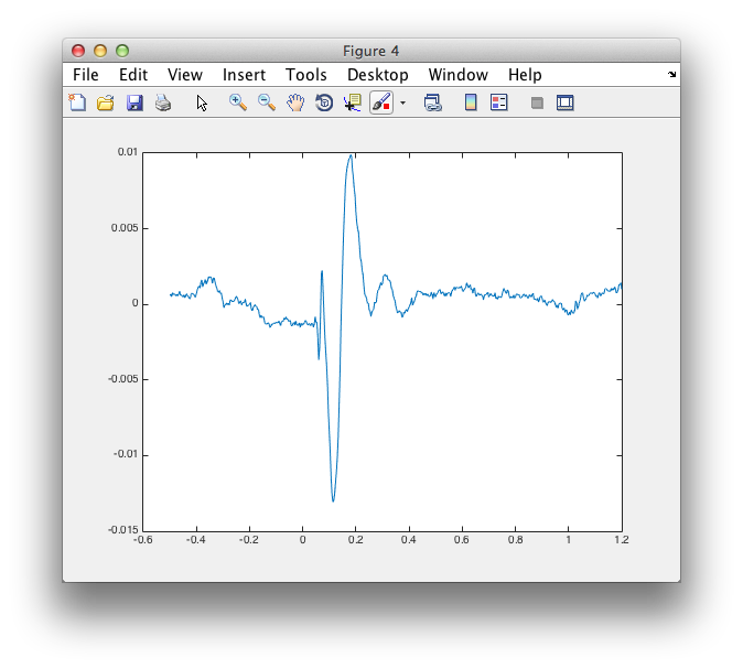
source = ft_sourceanalysis(cfg, timelock2);

figure
plot(source.time, source.avg.mom{1})

%% construct single-trial virtual channel data

virtualchannel_raw = [];
virtualchannel_raw.label = {'source'};
virtualchannel_raw.trialinfo = data_fix.trialinfo;
for i=1:882
% note that this is the non-filtered raw data
virtualchannel_raw.time{i}       = data_fix.time{i};
virtualchannel_raw.trial{i}(1,:) = source.avg.filter{1} * data_fix.trial{i}(:,:);
end

%% average the virtual channel ERP

cfg = [];
cfg.keeptrials = 'yes';
cfg.preproc.demean = 'yes';
cfg.preproc.baselinewindow = [-inf 0];
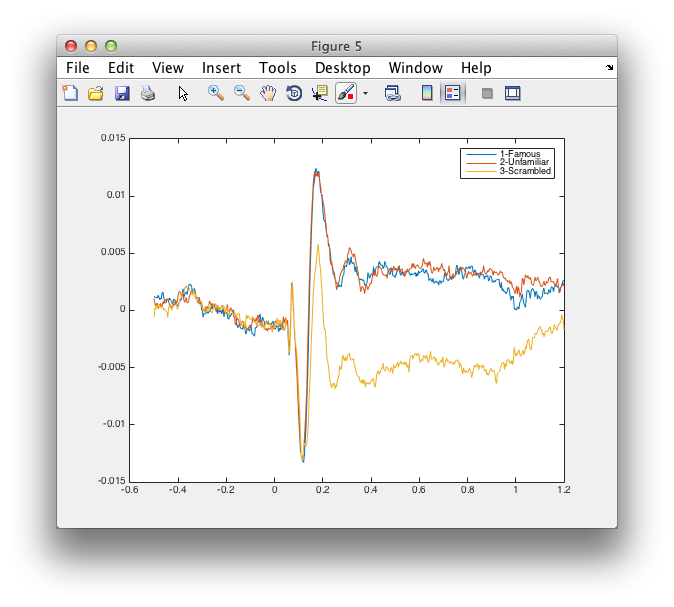
virtualchannel_avg = ft_timelockanalysis(cfg, virtualchannel_raw);
cfg.trials = virtualchannel_raw.trialinfo==1;
virtualchannel_avg1 = ft_timelockanalysis(cfg, virtualchannel_raw);
cfg.trials = virtualchannel_raw.trialinfo==2;
virtualchannel_avg2 = ft_timelockanalysis(cfg, virtualchannel_raw);
cfg.trials = virtualchannel_raw.trialinfo==3;
virtualchannel_avg3 = ft_timelockanalysis(cfg, virtualchannel_raw);

figure
plot(virtualchannel_avg.time, virtualchannel_avg.avg);

figure
plot(virtualchannel_avg.time, [virtualchannel_avg1.avg; virtualchannel_avg2.avg; virtualchannel_avg3.avg]);
legend({'1-Famous', '2-Unfamiliar', '3-Scrambled'})

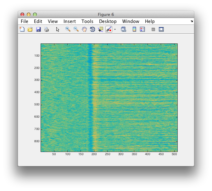
figure
imagesc(squeeze(virtualchannel_avg.trial))

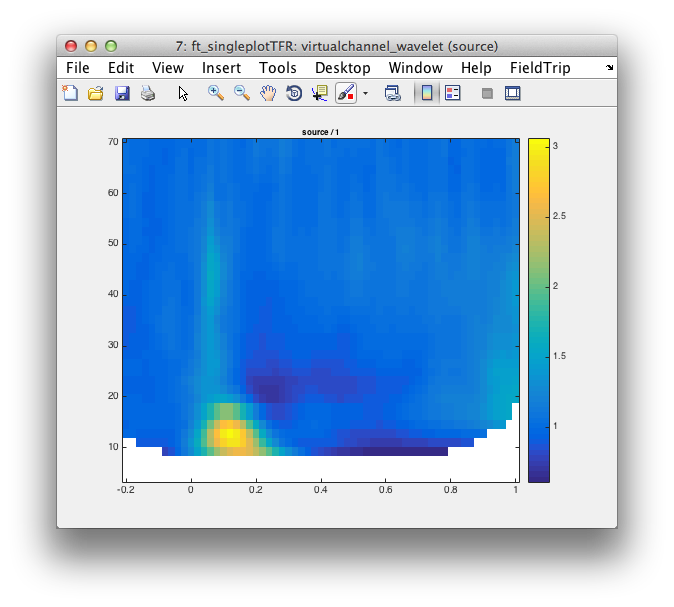
%% investigate the virtual channel spectrally

cfg = [];
cfg.method = 'wavelet';
cfg.output = 'pow';
cfg.foi = 4:2:70;
cfg.toi = -0.200:0.020:1.000;
virtualchannel_wavelet = ft_freqanalysis(cfg, virtualchannel_raw);

cfg = [];
cfg.baseline = [-inf 0];
cfg.baselinetype = 'relative';
cfg.interactive = 'no';
ft_singleplotTFR(cfg, virtualchannel_wavelet);