Preprocessing and event-related potentials in EEG data

Introduction

This tutorial describes how to define epochs of interest (trials) from recorded EEG data, and how to apply different preprocessing steps such as filtering, cleaning data and re-referencing electrodes. Subsequently, we will average our epochs/trials and acquire so-called event-related potentials (ERPs). We will also compare two different types of stimuli (standard versus deviant tones) and investigate the differing ERPs they give rise to.

In this tutorial, preprocessing and segmenting the data into epochs/trials are done in a single step. If you are interested in how to do preprocessing on continuous data prior to segmenting it into epochs/trials, you can check the Preprocessing - Reading continuous data tutorial.

Background

In FieldTrip, the preprocessing of data refers to the reading of the data, segmenting the data around interesting events, which are defined by triggers in the data, temporal filtering and (optionally) re-referencing. The ft_preprocessing function takes care of all these steps, i.e., it reads the data and applies the preprocessing options.

There are largely two alternative approaches for preprocessing, which especially differ in the amount of memory required.

1. Read all data from the file into memory, apply filters, and subsequently cut the data into interesting segments
2. Identify the interesting segments, read those segments from the data file and apply filters to those segments only

An advantage of the first approach is that it allows you to apply most temporal filters to your data without the distorting the data. In the latter approach, you have to be more careful with the temporal filtering you apply, but it is much more memory-friendly, especially for big datasets. Here we are using the second approach. The approach for reading and filtering continuous data and segmenting afterwards is explained in another tutorial.

We are going to define segments of interest (epochs/trials) based on triggers encoded in a specific trigger channel. This depends on the function ft_definetrial. The output of ft_definetrial is a so-called configuration structure (typically called cfg), which contains the field cfg.trl. This is a matrix representing the relevant parts of the raw data, which are to be selected for further processing. Each row in trl matrix represents a single epoch-of-interest (trial), and the trl matrix has three or more columns. The first column defines (in samples) the beginning point of each epoch with respect to how the data are stored in the raw data file. The second column defines (in samples) the end point of each epoch. The third column specifies the offset (in sample) of the first sample within each epoch with respect to time point 0 within than epoch. In essence they contain information about when the epoch begins, end and when time 0 appears. The trial matrix can contain more columns with more (user-chosen) information about the trial.

You can either use a default trial function or design your own. When using the default trial function, the fourth column will contain the trigger value of the trigger channel. If you do use your own trial function, you can add as many columns as you wish to the trl matrix, which will be contained in your segmented data in the .trialinfo field. Here, you can add information of for example response buttons, response times.

Details of the auditory oddball MEG+EEG Dataset

Please note that we will only be using the EEG data from this dataset.

For the 2014 EEG-MEG workshop at NatMEG we recorded a dataset of a single subject to allow you to work through all the different steps involved in EEG and MEG analysis: from event-related averaging to frequency analysis, source modeling and statistics.

The oddball paradigm

The experiment that the subject performed is a slight adaptation of the classical oddball experiment. Using the oddball paradigm one can study the well-known EEG component called the mismatch-negativity (MMN). The classical auditory oddball experiment involves the presentation of a continuous series of identical tones at a relatively slow rate, say between one every two seconds to two every second. Every so often, say one out of ten, the tone is slightly different in pitch, duration or loudness. In our version, an oddball occurs after every 3 to 7 standard tones. The interval between each tone is jittered between 700 to 900 ms.

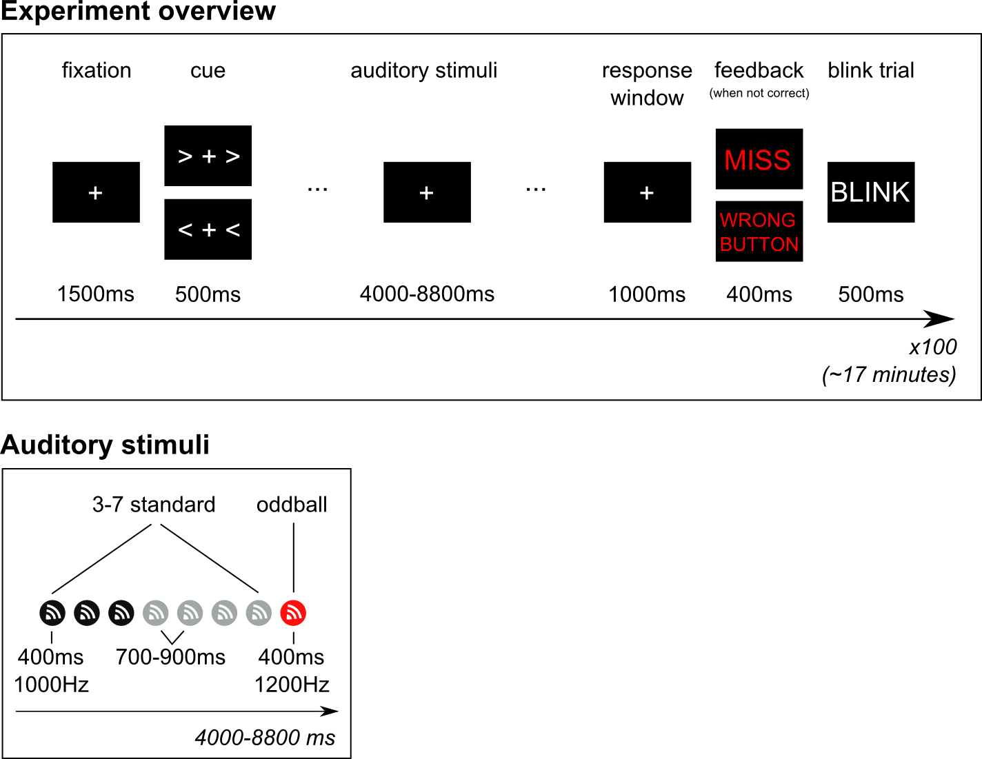
Mismatch negativity

The auditory MMN then occurs as a fronto-central negative EEG potential (relative to the response to the standard tone), with sources in the primary and non-primary auditory cortex and a typical latency of 150-250 ms after the onset of the deviant tone. Not only is the MMN an indicator or auditory functioning, it has also been shown to be under influence of cognitive factors and indicative of cognitive and psychiatric impairments. For a recent and comprehensive overview please see Näätänen et al (2007).

Cued motor preparation

For the purpose of analyzing oscillatory dynamics we wanted the oddball paradigm to include motor responses, specifically left and right button-presses with the left and right index finger, respectively. The subject was therefor cued to respond with their left or right index finger whenever, and as soon as possible, after a deviant tone occurred. The experiment therefore consistent of series of standard tones + deviant, preceded by a cue (left or right), and followed by a button-press.

Beta suppression and rebound

It is well known that power in the beta band (15–30 Hz) decreases prior to movement onset but showed a marked sudden increase beginning approximately 300 to 400 ms after termination of EMG activity and lasting for over 500 ms. This post-movement beta rebound (PMBR) is localized to bilateral regions of the pre-central gyrus, but with greater lateralization to the contralateral hemisphere. Contrasting left versus right responses should therefor give us a nice lateralized beta rebound in the pre-central gyrus.

For a recent overview of sensorimotor rhythms, including the beta rebound, please see Cheyne (2013).

Training with feedback and blink trials

Before the recording, the subject performed the experiment in a short training session to get acquainted with the task. Whenever the subject was too late in responding (>2 seconds), or pressed the wrong button, feedback was provided. In the actual experiment the subject was always on time and responded with the correct hand each time.

Finally, after each response, a blink trial is presented in which subjects are asked to blink so that they can remain fixated on the fixation cross - without blinking - throughout the period in time in which we are interested in the brain signal.

Stimuli

The standard tones were 400ms 1000Hz sine-waves, with a short 50ms ramping up- and down to avoid a clicking sound. The oddball tones were identical except for being 1200Hz. The auditory stimuli are presented with an external device that stores uncompressed audio files (.wav) that can then be presented with sub-millisecond precision (in effect instantaneous). Sound was presented through flat-panel sound showers. We measured the duration between the arrival of the triggers (see below) in the data and the arrival of the sound through the air to the ears of the subject. This takes 7.0 ms.

Triggers

The MEG system records event-triggers in a separate channels, called STI101 and STI102. These channels are recorded simultaneously with the data channels, and at the same sampling rate. The onset (or offset) can therefore be precisely timed with respect to the data. The following trigger codes can be used for the analysis we will be doing during the workshop:

• Onset of standard stimulus: 1
• Onset of oddball stimulus: 2
• Button-press onset of left hand: 256
• Button-press onset of right hand: 4096

Data

• Data was sampled at 1000Hz.
• 306 channels MEG of which 102 are magnetometers, and 204 are planar gradiometers.
• 128 electrode EEG. The reference was placed on the right mastoid, the ground on the left mastoid. The locations of the electrodes are placed according to the 5% system, which is an extension of the standard 10-20 system for high-density EEG caps. You can find details in Oostenveld and Praamstra, (2001). In addition, the locations of the EEG electrodes was measured in 3D using the Polhemus system and recorded in the data.
• Horizontal EOG(1) electrodes were placed just outside the left and right eye. Vertical EOG(2) were placed above and below the left eye.
• Electrocardiogram (ECG) was recorded as a bipolar recording from the collarbones.
• Electromyography of the lower arm flexors of the left(1) and right(2) arm were recorded.

Have a look at the data prior to preprocessing

Before we start preprocessing our data and calculate event-related potentials (ERPs), we will first have a look at our data while it is unprocessed and not yet cut into trial (following FieldTrip nomenclature: raw data). To do this, we use ft_databrowser. Note that ft_databrowser is very memory efficient, as it does not read all data into memory - only the part that it displays.

How can I use the data browser?

The data browser can be used to look at your raw or preprocessed data. The main purpose is to do quality checks and visual artifact detection and also annotate time periods during which specific artifacts happens. However, it also supports annotation of the data, such as annotating sleep spindles or epileptic spikes.

The data browser supports three view modes: butterfly, vertical and component. In butterfly, all signal traces will be plotted on top of one another; in vertical, the traces will be below one another. The component view mode is to be used for data that is decomposed into independent components (see ft_componentanalysis. Components will be plotted as in the vertical view mode, but will include the component topography to the left of the time trace. As an alternative to these three view modes, you can provide a cfg.layout, and ft_databrowser will try to plot the data according to the sensor positions specified in that layout.

When the data browser opens, you will see button to navigate along the bottom of the screen and buttons for artifact annotation to the right. Note that also artifacts that were marked with automatic artifact detection methods will be displayed here (see the automatic artifact rejection tutorial). You can click on one of the artifact types, drag over a time window to select the beginning and the end of the artifact and then double-click in the selected area to mark it as an artifact. Double-clicking again will remove the selection.

Before we begin

We will clear all variables that we have in the workspace, restore the default path, add fieldtrip and run ft_defaults

clear variables
restoredefaultpath

addpath /home/lau/matlab/fieldtrip/ %% set your own path
ft_defaults

Visualization of raw EEG data

The EEG dataset used in this tutorial is available here

cfg            = [];
cfg.dataset    = 'oddball1_mc_downsampled_eeg.eeg';
cfg.continuous = 'yes';
cfg.viewmode   = 'vertical';
cfg.blocksize  = 1; % duration of data to display, in seconds

ft_databrowser(cfg);

set(gcf, 'units', 'normalized', 'outerposition', [0 0 1 1]) % full screen
print -dpng databrowser_oslo2019.png

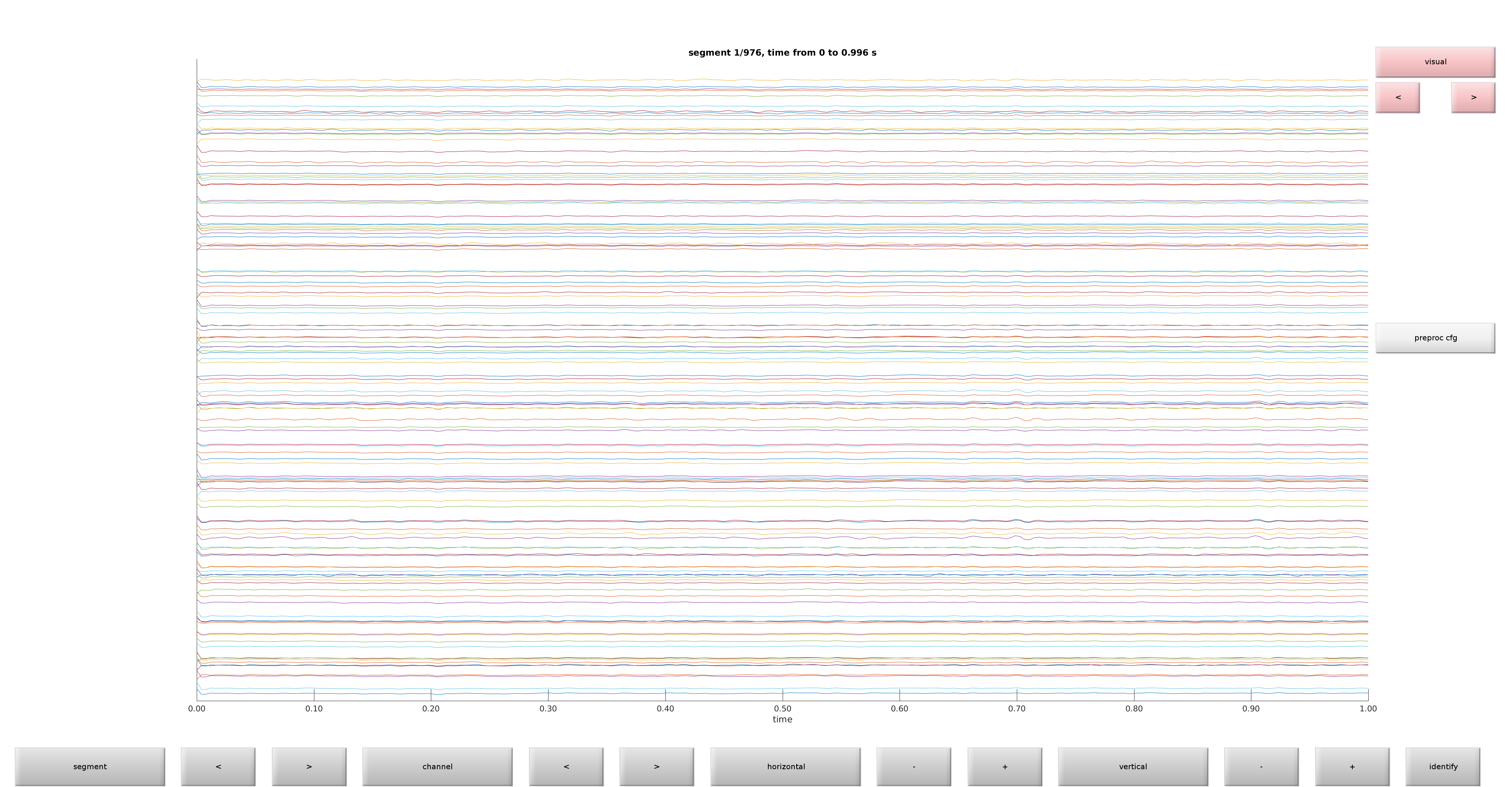
Figure 1: Raw plot of electrodes using ft_databrowser

Preprocessing and averaging EEG

In this step, we will preprocess and subsequently average our epochs/trials to obtain ERPs.

Procedure

We will take the following steps

• Define segments of data of interest (the trial definition) using ft_definetrial
• Read the data into MATLAB using ft_preprocessing
• Clean the data in a semi-automatic way using ft_rejectvisual
• Calculate event-related potentials (ERPs) using ft_timelockanalysis
• Visualize the results using ft_multiplotER, ft_singleplotER and ft_topoplotER

Reading and preprocessing the epochs/trials of interest

cfg = [];
cfg.dataset             = 'oddball1_mc_downsampled_eeg.vhdr';

cfg.trialdef.eventtype  = 'STI101'; % name of trigger channel
cfg.trialdef.eventvalue = {1 2}; % 1 is standard, 2 is deviant
cfg.trialdef.prestim    = 0.200; % seconds
cfg.trialdef.poststim   = 0.600; % seconds
cfg.trialfun = 'ft_trialfun_general';

cfg = ft_definetrial(cfg); %% note that a new cfg is created here

% and we add more stuff to it here

cfg.continuous          = 'yes';    % data is continuous
cfg.hpfilter            = 'no';     % we do not apply a high-pass filter
cfg.detrend             = 'no';     % we do not detrend
cfg.demean              = 'yes';    % we demean (baseline correct) ...
cfg.baselinewindow      = [-Inf 0]; % using the mean activity in this window
cfg.dftfilter           = 'yes';    % a notch filter ...
cfg.dftfreq             = [50 100]; % hitting the (European) power frequency
                                    % (and its first harmonic)
cfg.channel             = 'EEG';

cfg.reref               = 'yes';    % was recorded with left mastoid but is ...
cfg.refchannel          = 'all';    % re-referenced to all (also called common average

data                    = ft_preprocessing(cfg);

The output of ft_preprocessing(cfg) is data, which is a structure that has the following fields:

data =

           hdr: [1x1 struct]
         label: {128x1 cell}
          time: {1x600 cell}
         trial: {1x600 cell}
       fsample: 250
    sampleinfo: [600x2 double]
     trialinfo: [600x1 double]
           cfg: [1x1 struct]

• hdr contains header information about the data structure (metadata)
• label contains the names of all channels
• time contains the time courses for each of the 600 trials
• trial contains the voltages for each of the 600 trials
• fsample indicates the sampling frequency in Hz
• sampleinfo is a matrix the samples at which sample points trials begin and end
• trialinfo is a column vector indicating the type of trial (1=standard, 2=deviant)
• cfg contains information about the call leading to this output

Let’s have a closer look at the first entries in time and trial:

>> size(data.time{1})

ans =
     1   200

>> size(data.trial{1})

ans =
   128   200

• For time this is a row vector which has 200 entries, thus there are 200 time points in this epoch
• For trial this is a matrix with 128 rows and 200 columns, having the voltage for each of the 128 channels and the 200 time points

Cleaning data using visual summaries

In this tutorial, we are going to use a visual summary tool for rejecting bad trials. It is also possible to annotate artifacts using a more automatic procedure (see the automatic artifact rejection tutorial).

cfg        = [];
cfg.layout = 'natmeg_customized_eeg1005.lay';

cleaned_data_ERP = ft_rejectvisual(cfg, data);

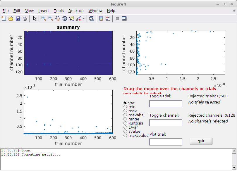
Figure 2: The visual summary plot tool

You can use different metrics to calculate the summary, but variance is usually a good metric.

In my case, I removed 26 trials

cleaned_data_ERP =

           hdr: [1x1 struct]
         label: {128x1 cell}
          time: {1x574 cell}
         trial: {1x574 cell}
       fsample: 250
    sampleinfo: [574x2 double]
     trialinfo: [574x1 double]
           cfg: [1x1 struct]

If you want to carry on with the data cleaned by the organizers, load the data using the command below.

load cleaned_data_ERP.mat

Event-Related Potentials (ERPs) (also unfortunately known as time-locked responses)

The function ft_timelockanalysis makes an average (ERP) over all the trials in a segmented data structure. For purposes of visualization, we will also apply a low-pass filter. Note that we could have done that earlier as well, but rather we decided to clean before applying low- or high-pass filters.

cfg                = [];
cfg.lpfilter       = 'yes';
cfg.lpfreq         = 30;
cfg.detrend        = 'yes';     % removing linear trends
cfg.baselinewindow = [-Inf 0];  % using the mean activity in this window

data_EEG_filt = ft_preprocessing(cfg, cleaned_data_ERP);

We are creating two ERPs, one for the standard and one for the deviant.

cfg          = [];
cfg.trials   = find(data_EEG_filt.trialinfo == 1);
ERP_standard = ft_timelockanalysis(cfg, data_EEG_filt);

cfg         = [];
cfg.trials  = find(data_EEG_filt.trialinfo == 2);
ERP_deviant = ft_timelockanalysis(cfg, data_EEG_filt);

The output of ft_timelockanalysis looks like this:

ERP_standard =

      time: [1x200 double]
     label: {128x1 cell}
       avg: [128x200 double]
       var: [128x200 double]
       dof: [128x200 double]
    dimord: 'chan_time'
       cfg: [1x1 struct]

• time is now just a row vector with the time points in seconds (before we had a cell array with 600 cells in it)
• label is still our 128 names
• avg contains our averages for each of the 128 channels at each of the 200 time points
• var contains the variance for each of the 128 channels at each of the 200 time points (can be used e.g., for calculating standard deviations)
• dof contains the degrees of freedoms for each of the 128 channels at each of the 200 time points
• dimord indicates the ordering of dimensions, rows are channels and columns are time
• cfg shows the cfg that gave rise to this structure

These can be plotted using ft_multiplotER, ft_singleplotER and ft_topoplotER

Multiplot

cfg        = [];
cfg.layout = 'natmeg_customized_eeg1005.lay';

figure
ft_multiplotER(cfg, ERP_standard, ERP_deviant);

print -dpng multiplot.png

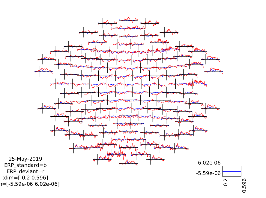
Figure 3: A plot of all channels

Singleplot

cfg         = [];
cfg.layout  = 'natmeg_customized_eeg1005.lay';
cfg.channel = 'EEG124';
cfg.ylim    = [-5e-6 5e-6]; % Volts

figure
ft_singleplotER(cfg, ERP_standard, ERP_deviant);

hold on
xlabel('Time (s)')
ylabel('Electric Potential (V)')
plot([ERP_standard.time(1), ERP_standard.time(end)], [0 0], 'k--') % add horizontal line
plot([0 0], cfg.ylim, 'k--') % vert. l
legend({'Standard', 'Deviant'})

print -dpng singleplot.png

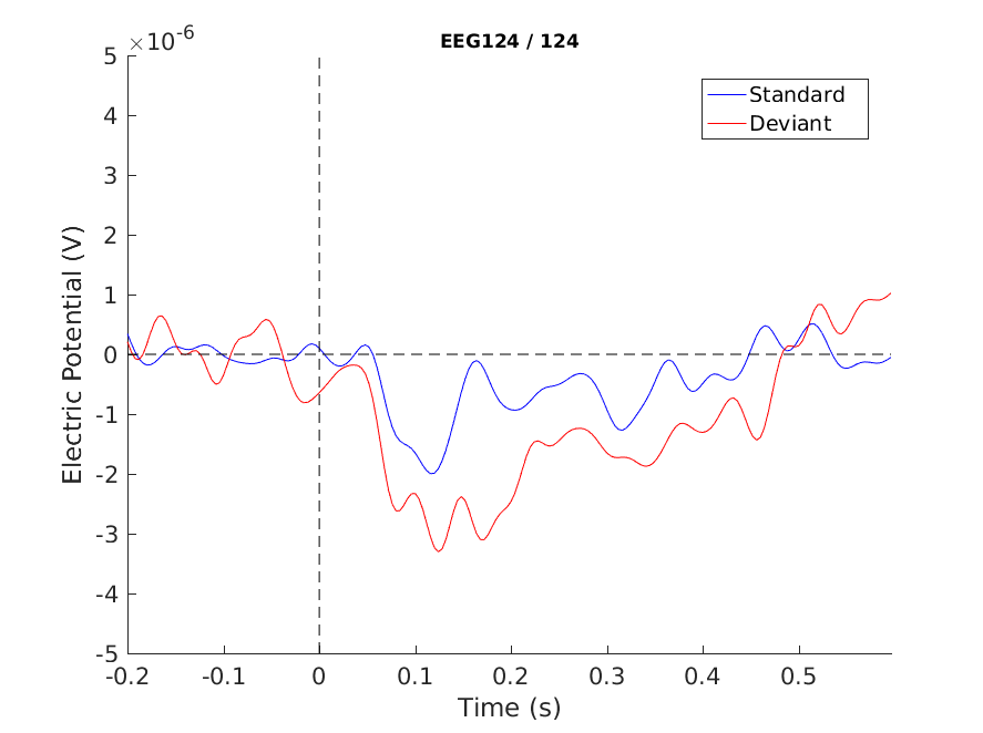
Figure 4: A plot of a single channel

Topoplot

figure

cfg              = [];
cfg.layout       = 'natmeg_customized_eeg1005.lay';
cfg.xlim         = [0.100 0.170]; % seconds
cfg.zlim         = [-4e-6 4e-6]; % Volts
cfg.colorbar     = 'yes';
cfg.colorbartext =  'Electric Potential (V)';

ft_topoplotER(cfg, ERP_standard);
title('Auditory Response: Standard')
print -dpng standard_aud.png

figure
ft_topoplotER(cfg, ERP_deviant);
title('Auditory Response: Deviant')
print -dpng deviant_aud.png

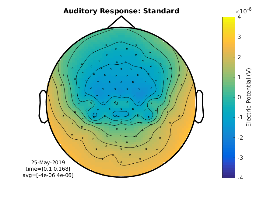
Figure 5: A topographical plot showing the average electric potential between 100 and 170 ms for the standard

Figure 6: A topographical plot showing the average electric potential between 100 and 170 ms for the deviant

Difference Wave

We can calculate the difference wave, the subtraction of one ERP from another

cfg           = [];
cfg.operation = 'x2-x1';
cfg.parameter = 'avg';

difference_wave = ft_math(cfg, ERP_standard, ERP_deviant);

These can be plotted using the same tools as before

Multiplot

cfg        = [];
cfg.layout = 'natmeg_customized_eeg1005.lay';

figure
ft_multiplotER(cfg, difference_wave);

print -dpng multiplot_diff.png

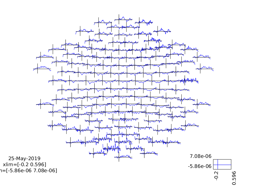
Figure 7: A plot of all channels showing the MMN

cfg         = [];
cfg.layout  = 'natmeg_customized_eeg1005.lay';
cfg.channel = 'EEG124';
cfg.ylim    = [-5e-6 5e-6]; % Volts

figure
ft_singleplotER(cfg, difference_wave);

hold on
xlabel('Time (s)')
ylabel('Difference in Electric Potential (V)')
plot([ERP_standard.time(1), ERP_standard.time(end)], [0 0], 'k--') % add horizontal line
plot([0 0], cfg.ylim, 'k--') % vert. l

print -dpng singleplot_MMN.png

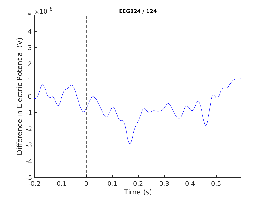
Figure 8: A plot of a single channel showing the MMN

cfg              = [];
cfg.layout       = 'natmeg_customized_eeg1005.lay';
cfg.xlim         = [0.100 0.170]; % seconds
cfg.zlim         = [-1.5e-6 1.5e-6]; % Volts
cfg.colorbar     = 'yes';
cfg.colorbartext =  'Electric Potential Difference (V)';

figure
ft_topoplotER(cfg, difference_wave);
title('Mismatch Negativity (MMN)')

print -dpng MMN.png

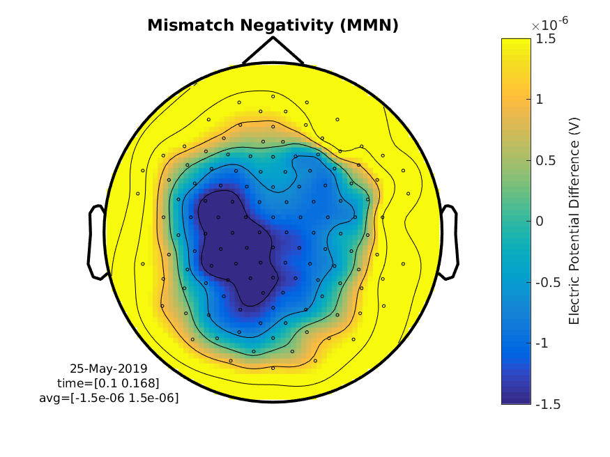
Figure 9: A topographical plot showing the MMN (average over 100 to 170 ms)

Bonus: Visualize the temporal evolution of the ERP as a movie

figure

cfg        = [];
cfg.layout = 'natmeg_customized_eeg1005.lay';

ft_movieplotER(cfg, difference_wave);

Play around with the zlim to get a feeling for how the difference_wave changes topography. Try also plotting the the ERPs themselves.