workshop / oslo2019 / statistics /
Statistical analysis and multiple comparison correction for EEG data
Introduction
The objective of this tutorial is to give an introduction to the statistical analysis of EEG data using different methods to control for the false alarm rate. The tutorial starts with sketching the background of cluster-based permutation tests. Subsequently it is shown how to use FieldTrip to perform statistical analysis (including cluster-based permutation tests) on the time-frequency response to a movement, and to the auditory mismatch negativity. The tutorial makes use of a between-trials (within-subject) design.
In this tutorial we will continue working on the dataset described in the Preprocessing and event-related activity and the Time-frequency analysis of MEG and EEG tutorials. We will repeat some code here to select the trials and preprocess the data. We assume that the preprocessing and the computation of the ERFs/TFRs are already clear to the reader.
This tutorial is not covering group analysis. Look here for that. If you are interested, you can read the other tutorials that cover cluster-based permutation tests on event-related fields and on time-frequency data. If you are interested in a more gentle introduction as to how parametric statistical tests can be used with FieldTrip, you can read the Parametric and non-parametric statistics on event-related fields tutorial.
This tutorial contains the hands-on material of the NatMEG workshop. The background is explained in this lecture, which was recorded at the Aston MEG-UK workshop.
Background
The topic of this tutorial is the statistical analysis of multi-channel EEG data. In cognitive experiments, the data is usually collected in different experimental conditions, and the experimenter wants to know whether there is a difference in the data observed in these conditions. In statistics, a result (for example, a difference among conditions) is statistically significant if it is unlikely given the null hypothesis that there is no difference between the conditions. The “unlikeliness” is evaluated according to a predetermined threshold probability, the alpha level.
An important feature of EEG data is that it has spatio-temporal structure, i.e. the data is sampled at multiple time-points and sensors. The nature of the data influences which kind of statistics is the most suitable for comparing conditions. If the experimenter is interested in a difference in the signal at a certain time-point and sensor, then the more widely used parametric tests are sufficient. If it is not possible to predict where the differences are, then many statistical comparisons are necessary which lead to the multiple comparisons problem (MCP). The MCP arises from the fact that the effect of interest (i.e., a difference between experimental conditions) is evaluated at an extremely large number of (channel,time)-pairs. This number is usually in the order of several thousands. Now, the MCP involves that, due to the large number of statistical comparisons (one per (channel,time)-pair), it is not possible to control the so called family-wise error rate (FWER) by means of the standard statistical procedures that operate at the level of single (channel,time)-pairs. The FWER is the probability, under the hypothesis of no effect, of falsely concluding that there is a difference between the experimental conditions at one or more (channel,time)-pairs. A solution of the MCP requires a procedure that controls the FWER at some critical alpha-level (typically, 0.05 or 0.01). The FWER is also called the false alarm rate.
When parametric statistics are used, one method that addresses this problem is the so-called Bonferroni correction. The idea is if the experimenter is conducting n number of statistical tests then each of the individual tests should be tested under a significance level that is divided by n. The Bonferroni correction was derived from the observation that if n tests are performed with an alpha significance level then the probability that one test comes out significant is smaller than or equal to n times alpha (Boole’s inequality). In order to keep this probability lower, we can use an alpha that is divided by n for each test. However, the correction comes at the cost of increasing the probability of false negatives, i.e. the test does not have enough power to reveal differences among conditions.
In contrast to the familiar parametric statistical framework, it is straightforward to solve the MCP in the nonparametric framework. Nonparametric tests offer more freedom to the experimenter regarding which test statistics are used for comparing conditions, and help to maximize the sensitivity to the expected effect. For more details see the publication by Maris and Oostenveld (2007).
Procedure for ERPs
Before we begin
We will clear all variables that we have in the workspace, restore the default path, add fieldtrip and run ft_defaults
clear variables
restoredefaultpath

addpath /home/lau/matlab/fieldtrip/ %% set your own path
ft_defaults
Load the ERP data and preprocess
load cleaned_data_ERP.mat
load ERP_deviant.mat
load ERP_standard.mat
load difference_wave.mat
load elec.mat
First, we load the data that we created in the ERP tutorial
Note the naming convention used - each saved .mat-file contains one and only one variable, which has the same name as the .mat-file This makes it clear what variables are loaded into the workspace.
We then apply the same preprocessing as before.
cfg                = [];
cfg.lpfilter       = 'yes';
cfg.lpfreq         = 30;
cfg.demean         = 'yes'; % we demean (baseline correct) ...
cfg.detrend        = 'yes'; % removing linear trends
cfg.baselinewindow = [-Inf 0];% using the mean activity in this window

data_EEG_filt = ft_preprocessing(cfg, cleaned_data_ERP);
The Student’s t-test
A ubiquitous test used to assess statistical significance is the Student’s t-test Wikipedia entry original article. To perform the t-test, t-values need to be calculated, which a bit simplified are: \frac{µ}{SEM}, where µ is the mean difference between the conditions and SEM is the standard deviation divided by \sqrt{n}, where n is the number of observations.
We will do a within-subject between-trials statistical test. We proceed by computing the statistical test, which returns the t-value, the probability and a binary mask that contains a 0 for all data points where the probability is below the a-priori threshold, and 1 where it is above the threshold. The cfg.design field specifies the condition in which each of the trials is observed. For the indepsamplesT statistic, it should contain 1’s and 2’s.
cfg           = [];

cfg.method    = 'analytic'; % using a parametric test
cfg.statistic = 'ft_statfun_indepsamplesT'; % using independent samples
cfg.correctm  = 'no'; % no multiple comparisons correction
cfg.alpha     = 0.05;

cfg.design    = data_EEG_filt.trialinfo; % indicating which trials belong ...
                                         % to what category
cfg.ivar      = 1; % indicating that the independent variable is found in ...
                   % first row of cfg.design

stat_t = ft_timelockstatistics(cfg, data_EEG_filt);
stat_t contains:
stat_t =

       stat: [128x200 double]
         df: 572
    critval: [-1.9641 1.9641]
       prob: [128x200 double]
       mask: [128x200 logical]
     dimord: 'chan_time'
       elec: [1x1 struct]
      label: {128x1 cell}
       time: [1x200 double]
        cfg: [1x1 struct]
- stat contains the t-values at all channels and time points
- df is the degrees of freedom determining the t-distribution that the t-value is compared against to obtain the p-values
- critval contains the critical values for the test performed; if a t-value is lesser than the negative value or greater than the positive value, the difference is declared significant. The critval is dependent on cfg.alpha and the degrees of freedom (df)
- prob contains the p-values associated with the t-values given the degrees of freedom (df)
- mask is a logical matrix, 0’s are where p-values (prob) are greater than cfg.alpha, 1’s are where they are lesser than cfg.alpha
- dimord indicates the ordering of dimensions, rows are channels and columns are time
- elec contains information about the electrodes, e.g., positions and names
- label contains the names of all channels
- time is a row vector with the time points in seconds
- cfg shows the cfg that gave rise to this structure
We can now plot the ERPs using the field cfg.maskparameter of the plotting functions: ft_multiplotER, ft_singleplotER and ft_topoplotER
Here, we will show ft_singleplotER
ERP_standard.mask = stat_t.mask; % adding mask to ERP

figure

cfg               = [];
cfg.layout        = 'natmeg_customized_eeg1005.lay';
cfg.maskparameter = 'mask';
cfg.maskstyle     = 'box';
cfg.maskfacealpha = 0.5; % transparency of mask
cfg.channel       = 'EEG124';
cfg.ylim          = [-5e-6 5e-6]; % Volts

ft_singleplotER(cfg, ERP_standard, ERP_deviant);
hold on
xlabel('Time (s)')
ylabel('Electric Potential (V)')
plot([ERP_standard.time(1), ERP_standard.time(end)], [0 0], 'k--') % hor. line
plot([0 0], cfg.ylim, 'k--') % vert. l
axes = gca;
legend(axes.Children([10 3]), {'Standard', 'Deviant'})

print -dpng singleplot_t_uncorrected.png
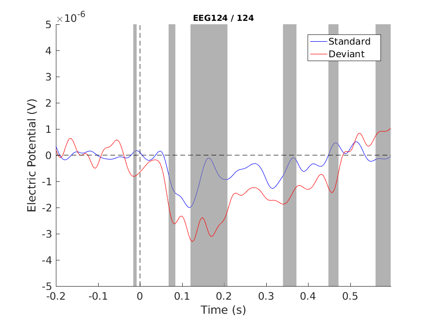
Figure 1: Single channel plot - no correction
Note that we see the MMN difference (~120-200 ms), but we also see other differences and even a pre-zero one. We cannot decide which are true positives and which are false positives. In fact, we know that there will be a lot false positives (assuming that the data were from identical distributions, i.e. the null hypothesis is true, we would expect that 5% of our significant differences are false positives)
Bonferroni correction
We will now control the false positives by using the Bonferroni Correction Wikipedia article
cfg           = [];

cfg.method    = 'analytic'; % using a parametric test
cfg.statistic = 'ft_statfun_indepsamplesT'; % using independent samples
cfg.correctm  = 'bonferroni'; % correction method
cfg.alpha     = 0.05;

cfg.design    = data_EEG_filt.trialinfo; % indicating which trials belong ...
                                         % to what category
cfg.ivar      = 1; % indicating that the independent variable is found in ...
                   % first row of cfg.design

stat_t_bonferroni = ft_timelockstatistics(cfg, data_EEG_filt);
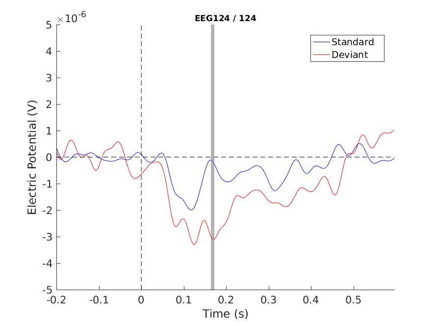
Figure 2: Single channel plot - Bonferroni correction
The Bonferroni correction has eliminated some likely false positives, but probably at the expense of introducing some false negatives. According to our image, only the peak of our MMN is significant. But EEG responses are not peaky in nature, they wax and wane smoothly in time and are smeared out over several electrodes. The Bonferroni correction implicitly assumes that EEG responses are uncorrelated, which they are patently not. Our next correction, the cluster correction addresses the issue of correlation.
Cluster-based correction for multiple comparisons
As noted above, EEG data is smooth over the spatio-temporal dimensions. We can easily imaging how we can build clusters in the temporal dimension. These are simply data points that are neighbouring each other in time. For the spatial dimension, it is necessary to build a neighbour structure using ft_prepare_neighbours. This uses the (digitized) positions of the electrodes.
Neighbors
Sometimes we use the word ‘neighbour’ according to the British spelling and sometimes we use it as neighbor according to the American spelling.
cleaned_data_ERP.elec = elec; % add the elec structure

cfg          = [];
cfg.method   = 'triangulation';
cfg.feedback = 'yes'; % visualizes the neighbors

neighbors = ft_prepare_neighbours(cfg, cleaned_data_ERP);

print -dpng neighbor_structure.png
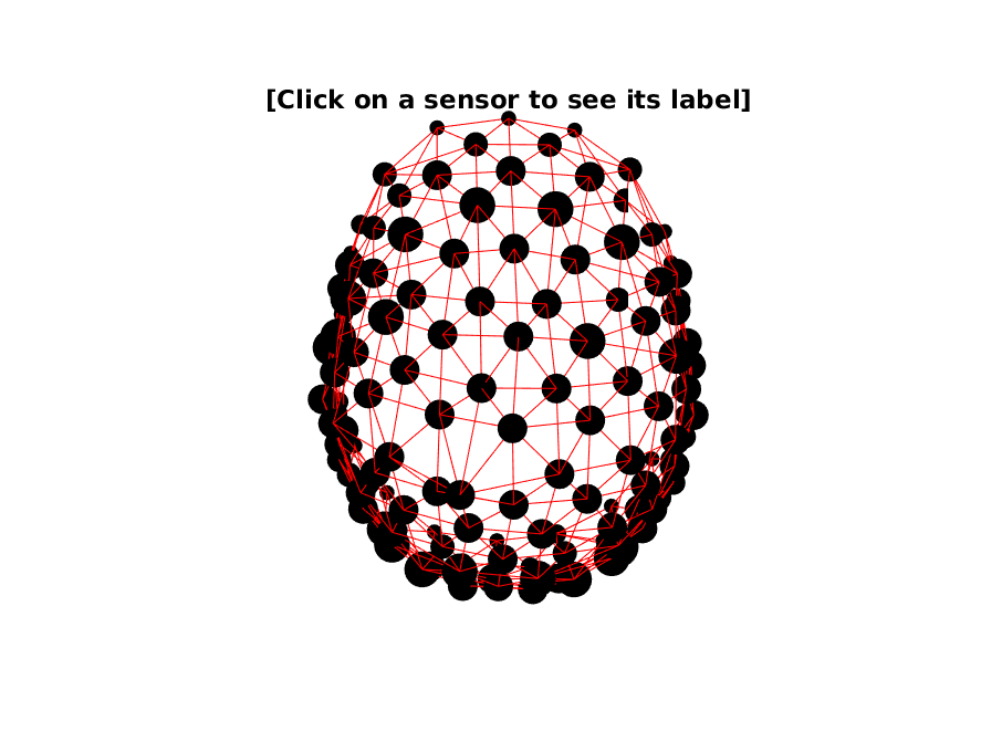
Figure 3: Electrode neighbor structure
Permutation
The cluster correction is not meaningful for parametric statistics, e.g., t-tests, therefore we are going to use a non-parametric test. We will first run it and then discuss some of the options and details afterwards.
cfg                  = [];
cfg.method           = 'montecarlo'; % use montecarlo to permute the data
cfg.statistic        = 'ft_statfun_indepsamplesT'; % function to use when ...
                                                   % calculating the ...
                                                   % parametric t-values

cfg.correctm         = 'cluster'; % the correction to use
cfg.clusteralpha     = 0.05; % the alpha level used to determine whether or ...
                             % not a channel/time pair can be included in a ...
                             % cluster
cfg.alpha            = 0.025; % corresponds to an alpha level of 0.05, since ...
                              % two tests are made ...
                              % (negative and positive: 2*0.025=0.05)
cfg.numrandomization = 100;  % number of permutations run

cfg.design           = data_EEG_filt.trialinfo; % same design as before
cfg.ivar             = 1; % indicating that the independent variable is found in ...
                          % first row of cfg.design
cfg.neighbours       = neighbors; % the spatial structure
cfg.minnbchan        = 2; % minimum number of channels required to form a cluster

stat_t_cluster = ft_timelockstatistics(cfg, data_EEG_filt);
The output of stat_t_cluster is:
stat_t_cluster =

                   prob: [128x200 double]
            posclusters: [1x11 struct]
    posclusterslabelmat: [128x200 double]
        posdistribution: [1x100 double]
            negclusters: [1x14 struct]
    negclusterslabelmat: [128x200 double]
        negdistribution: [1x100 double]
                cirange: [128x200 double]
                   mask: [128x200 logical]
                   stat: [128x200 double]
                    ref: [128x200 double]
                 dimord: 'chan_time'
                  label: {128x1 cell}
                   time: [1x200 double]
                    cfg: [1x1 struct]
- prob contains the p-values for each channel/time pair inherited from the cluster that pair is part of
- posclusters contains a structure for each positive cluster found that contains
- prob contains the p-value associated with the cluster
- clusterstat contains the T-value associated with this cluster
- stddev contains the standard deviation of the prob of this cluster
- cirange contains the 95% confidence interval for the prob of thus cluster - if this range include cfg.alpha a warning is issued recommending increasing the number of permutations
- posclusterslabelmat contains a matrix with a number indicating which positive cluster each channel/time pair belongs (0 if it doesn’t belong to
- posdistribution contains a row vector containing the T-value for each of the permutations
- negclusters contains the negative equivalent of posclusters
- negclusterslabelmat contains the negative equivalent of negclusterslabelmat
- negdistribution contains the negative equivalent of posdistribution
- cirange contains the 95% confidence interval for the prob
- mask is a logical matrix, 0’s are where p-values (prob) are greater than cfg.alpha, 1’s are where they are lesser than cfg.alpha
- stat contains the t-values (the first step)
- ref contains the mean value of the t-value over all of the permutations
- dimord indicates the ordering of dimensions, rows are channels and columns are time
- label contains the names of all channels
- time is a row vector with the time points in seconds
- cfg shows the cfg that gave rise to this structure
There’s quite a lot to unpack here. It is critical to distinguish between t-values and T-values here. We will now state the procedure step by step.
- Do a t-test similar to above (stat_t) - these provide the t-values in stat_t_cluster.stat
- Find the T-values for each cluster of t-values that pass the analytic significance test based on cfg.clusteralpha. The T-value for a cluster is the sum of all the t-values in that cluster
- Permute the condition labels (cfg.design) as many times as set in cfg.numrandomization; then compute the t-values (as in step 1 above), and compute the T-values for each of the clusters that pass the analytic significance test based on cfg.clusteralpha (as in step 2 above).
- For each of the cfg.numrandomization permutations, retrieve the maximum T-value, and create a permutation based distribution of T-values
- Observe the likelihood of the maximum T-value under the permuted distribution for the positive clusters direction and evaluate at cfg.alpha
- Repeat step 5 for the negative clusters
Below follows some figures and operations illustrating key features of these steps - (the code for these plots in the Appendix below)
Equivalence of the t-values (step 1)
>> isequal(stat_t.stat, stat_t_cluster.stat)

ans =

     1
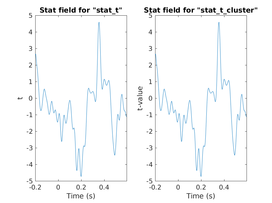
Figure 4: Equivalence of t-values
Cluster T-values (step 2)
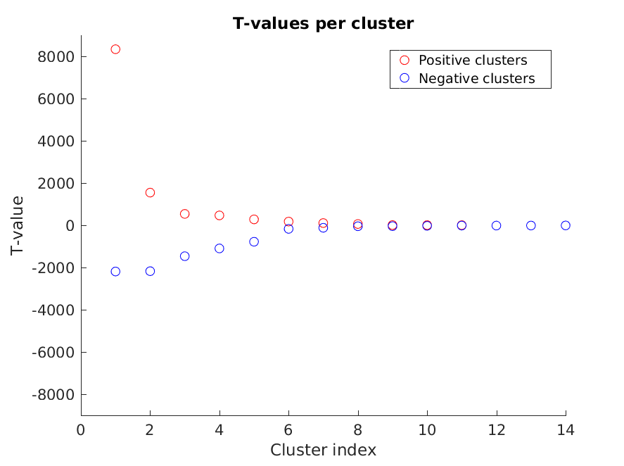
Figure 5: The T-values of each of the clusters
Maximum positive and negative cluster T-values compared to the permuted distributions (steps 3 and 4)
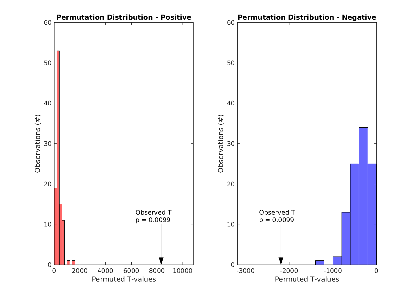
Figure 6: The observed positive and negative T-values compared to the permuted distributions
Compare against cfg.alpha (steps 5 and 6)
Since both the positive and negative p-values are lesser than cfg.alpha (0.025), we reject the null hypothesis for both the positive and negative directions. Put informally: our way of labelling the conditions does matter
Let’s have a look at the cluster corrected channel:
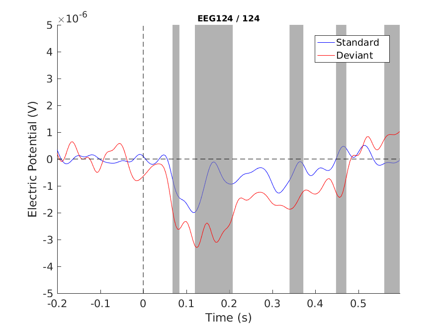
Figure 7: Single channel plot - Cluster correction
And here the three tested corrections are side by side
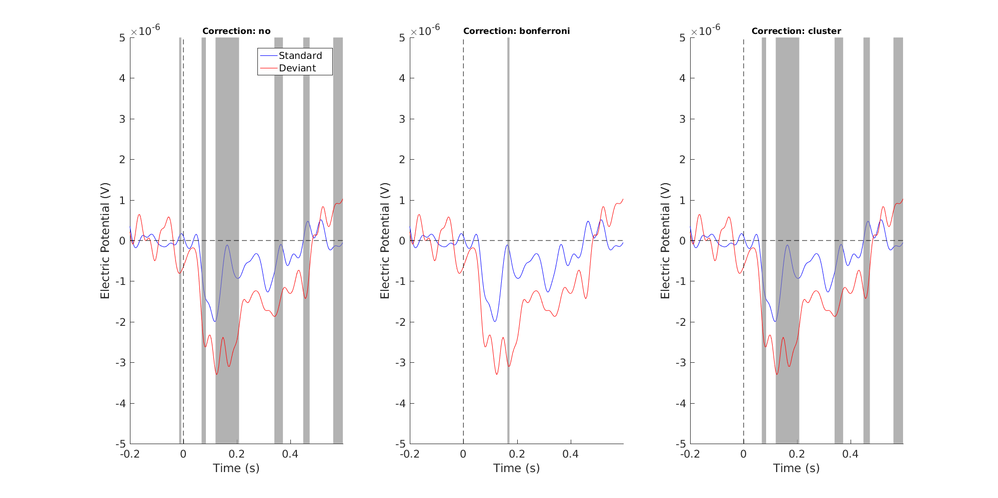
Figure 8: Single channel plot - corrections side by side
We can also do topographical plots. Here are the three side by side at 168 ms
n_plots = 3;
figure('units', 'normalized', 'outerposition', [0 0 0.5 0.5]);
stats = {stat_t stat_t_bonferroni stat_t_cluster};

for plot_index = 1:n_plots

    stat = stats{plot_index};
    subplot(1, 3, plot_index)

    difference_wave.mask = stat.mask;

    cfg               = [];
    cfg.layout        = 'natmeg_customized_eeg1005.lay';
    cfg.maskparameter = 'mask';
    cfg.xlim          = [0.168 0.168];
    cfg.zlim          = [-4.5e-6 4.5e-6]; % Volts
    if plot_index > 1;
        cfg.comment   = 'no';
    end

    ft_topoplotER(cfg, difference_wave)

    title(['Correction: ' stat.cfg.correctm])

end

print -dpng difference_wave_topoplots.png
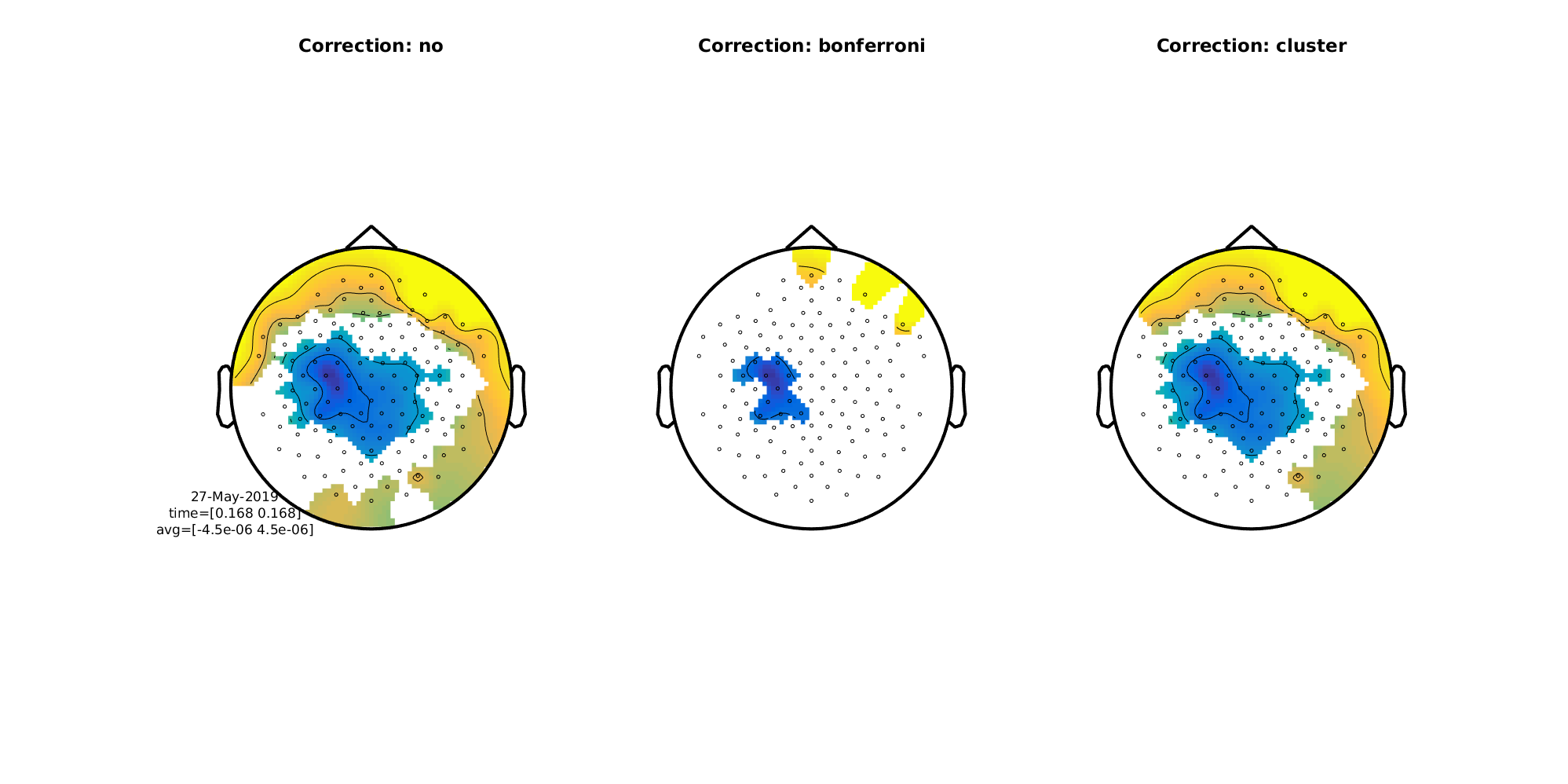
Figure 9: Difference wave (MMN) topographical plots
And here’s the difference between the normal t-mask and the t-cluster-mask. Note it is that not big.
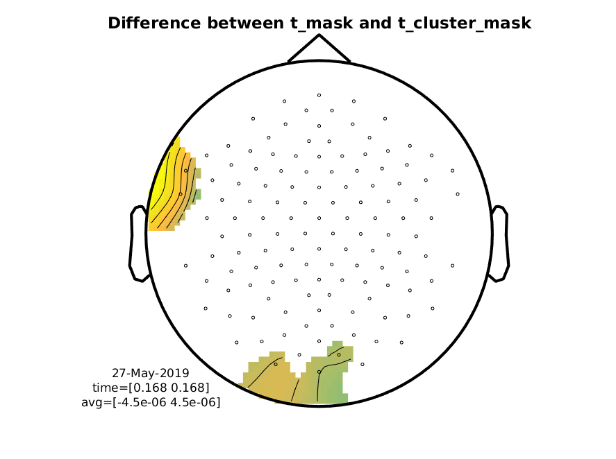
Figure 10: Difference wave showing the difference in masks coming from stat_t and stat_t_cluster
Do note that we, in EEG, most of the time do not make the inference at the level of the individual subject, but it is relevant to do so in for example diagnostic measurements.
We will now do a quick example of applying this to time-frequency data (TFR).
Procedure for TFRs
Here, we’ll just quickly show how to do within-subject statistics on TFRs
Load the data
First, we’ll load the data, both the ones with the trials and the ones with the average of the trials. We append the two trial data structures to one another using ft_appendfreq and we calculate the difference between the two averages using ft_math.
load tfr_left_trials.mat
load tfr_right_trials.mat
load tfr_left.mat
load tfr_right.mat

cfg = [];

tfr = ft_appendfreq(cfg, tfr_right_trials, tfr_left_trials);

cfg = [];
cfg.parameter    = 'powspctrm';
cfg.operation    = '(x1-x2) / (x1+x2)';

tfr_difference = ft_math(cfg, tfr_right, tfr_left);
We can see the sizes and ordering of dimensions using the in-built function size and checking the dimord
>> size(tfr.powspctrm)

ans =

   110   128    20    26

>> tfr.dimord

ans =

rpt_chan_freq_time
meaning that we have 110 trials on 128 channels at 20 frequencies and at 26 time points. For the difference between the averages, we have:
>> size(tfr_difference.powspctrm)

ans =

   128    20    26

>> tfr_difference.dimord

ans =

chan_freq_time
meaning that we have a difference between averages on 128 channels at 20 frequencies and at 26 time points.
Applying the tests
Note that we here apply the tests on the frequency range between 15 Hz and 30 Hz (the beta band range) and on the time interval between 400 ms and 1,000 ms (the time range of the beta rebound). This is set using cfg.frequency and cfg.latency. We do this because we have a priori knowledge that it is around here we should observe our beta rebound.
t-test with no correction
cfg           = [];
cfg.method    = 'analytic'; % using a parametric test
cfg.statistic = 'ft_statfun_indepsamplesT'; % using independent samples
cfg.correctm  = 'no'; % no multiple comparisons correction
cfg.alpha     = 0.05;
cfg.frequency = [15 30];
cfg.latency   = [0.400 1.000];

cfg.design    = zeros(1, length(tfr.trialinfo));
cfg.design(tfr.trialinfo == 256)  = 1; % indicating which trials belong ...
cfg.design(tfr.trialinfo == 4096) = 2; % to what category

cfg.ivar      = 1; % indicating that the independent variable is found in ...
                   % first row of cfg.design

stat_t_freq = ft_freqstatistics(cfg, tfr);
t-test with Bonferroni correction
cfg           = [];
cfg.method    = 'analytic'; % using a parametric test
cfg.statistic = 'ft_statfun_indepsamplesT'; % using independent samples
cfg.correctm  = 'bonferroni'; % no multiple comparisons correction
cfg.alpha     = 0.05;
cfg.frequency = [15 30];
cfg.latency   = [0.400 1.000];

cfg.design    = zeros(1, length(tfr.trialinfo));
cfg.design(tfr.trialinfo == 256)  = 1; % indicating which trials belong ...
cfg.design(tfr.trialinfo == 4096) = 2; % to what category

cfg.ivar      = 1; % indicating that the independent variable is found in ...
                   % first row of cfg.design

stat_t_bonferroni_freq = ft_freqstatistics(cfg, tfr);
Permutation test with cluster correction
cfg                  = [];
cfg.method           = 'montecarlo'; % use montecarlo to permute the data
cfg.statistic        = 'ft_statfun_indepsamplesT'; % function to use when ...
                                                   % calculating the ...
                                                   % parametric t-values
cfg.alpha            = 0.025; % corresponds to an alpha level of 0.05, since ...
                              % two tests are made ...
                              % (negative and positive: 2*0.025=0.05)
cfg.frequency = [15 30];
cfg.latency   = [0.400 1.000];

cfg.correctm         = 'cluster'; % the correction to use
cfg.clusteralpha     = 0.05; % the alpha level used to determine whether or ...
                             % not a channel/time pair can be included in a ...
                             % cluster
cfg.clustertail      = 0; % two-way t-test
cfg.clusterstatistic = 'maxsum';

cfg.numrandomization = 1000;  % number of permutations run

cfg.design    = zeros(1, length(tfr.trialinfo));
cfg.design(tfr.trialinfo == 256)  = 1; % indicating which trials belong ...
cfg.design(tfr.trialinfo == 4096) = 2; % to what category
cfg.ivar             = 1; % indicating that the independent variable is found in ...
                          % first row of cfg.design
cfg.neighbours       = neighbors; % the spatial structire
cfg.minnbchan        = 2; % minimum number of channels required to form a cluster

stat_t_cluster_freq = ft_freqstatistics(cfg, tfr);
Plotting the test results
stats = {stat_t_freq stat_t_bonferroni_freq stat_t_cluster_freq};
n_tests = length(stats);
h = figure;
for test_index = 1:n_tests

    subplot(1, 3, test_index)
    stat = stats{test_index};

    cfg = [];
    cfg.frequency = [stat.freq(1) stat.freq(end)];
    cfg.latency   = [stat.time(1) stat.time(end)];

    this_tfr = ft_selectdata(cfg, tfr_difference);

    this_tfr.mask = stat.mask;

    cfg = [];
    cfg.layout = 'natmeg_customized_eeg1005.lay';
    cfg.parameter = 'powspctrm';
    cfg.maskparameter = 'mask';
    cfg.maskstyle = 'outline';

    ft_multiplotTFR(cfg, this_tfr);
    c = colorbar('location', 'southoutside');
    c.Label.String = 'Power ratio (right over left)';
    title(['Correction: ' stat.cfg.correctm]);

end

set(h, 'units', 'normalized', 'outerposition', [0 0 1 1])
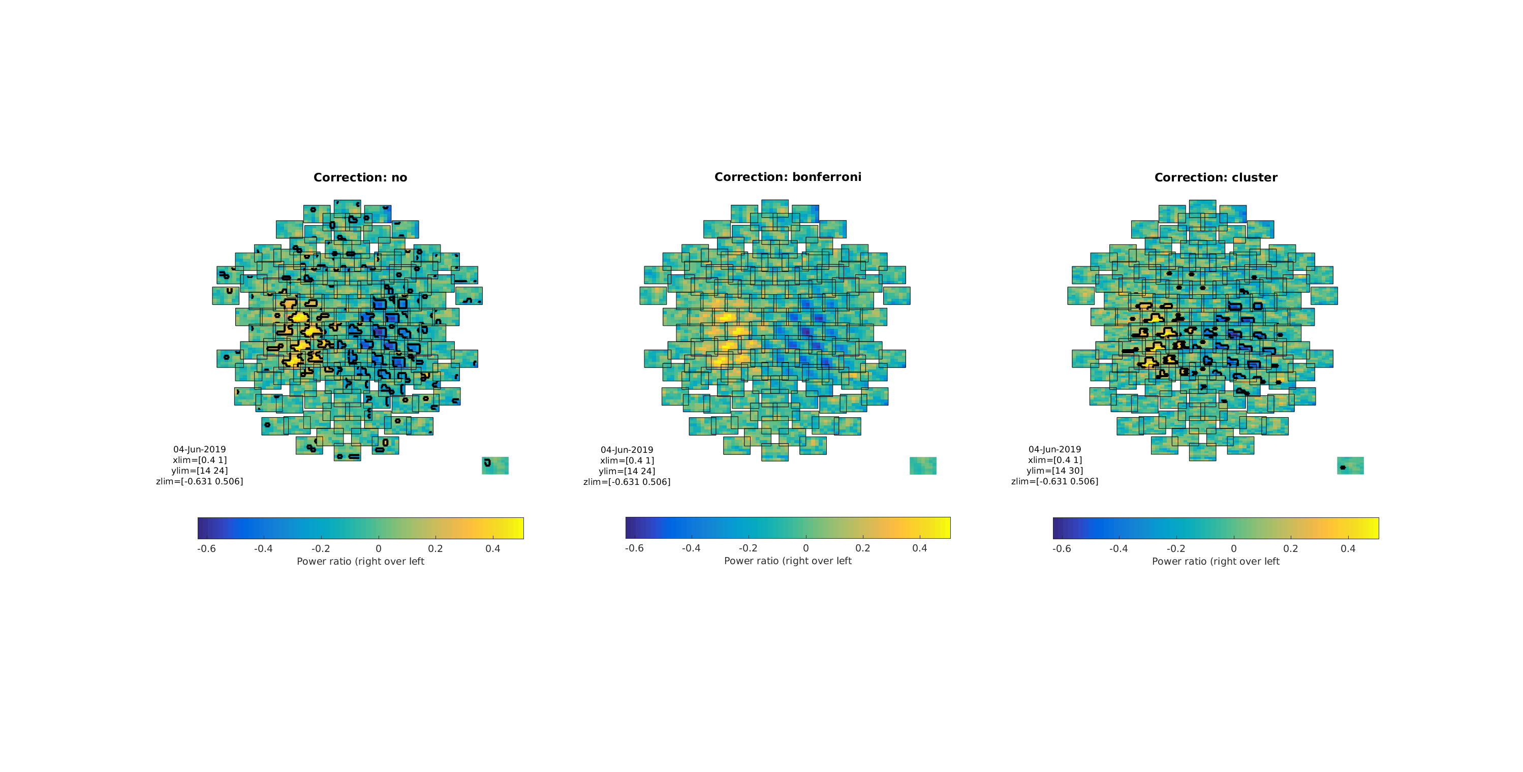
Figure 11: Three multiplots showing the differences between the three tests/corrections
Note how the cluster correction seems to catch the clusters that “catch” our eyes, while not showing the many non-clustered values that the non-corrected t-test showed. Also note that the Bonferroni correction removed all significant effects, showing that it is too conservative to apply to TFR data.
Extending the frequency and time ranges of the tests
Do the three tests again without setting cfg.frequency and cfg.latency (you can comment them out) Compare with the plot below - why may it be important to use one’s prior knowledge?
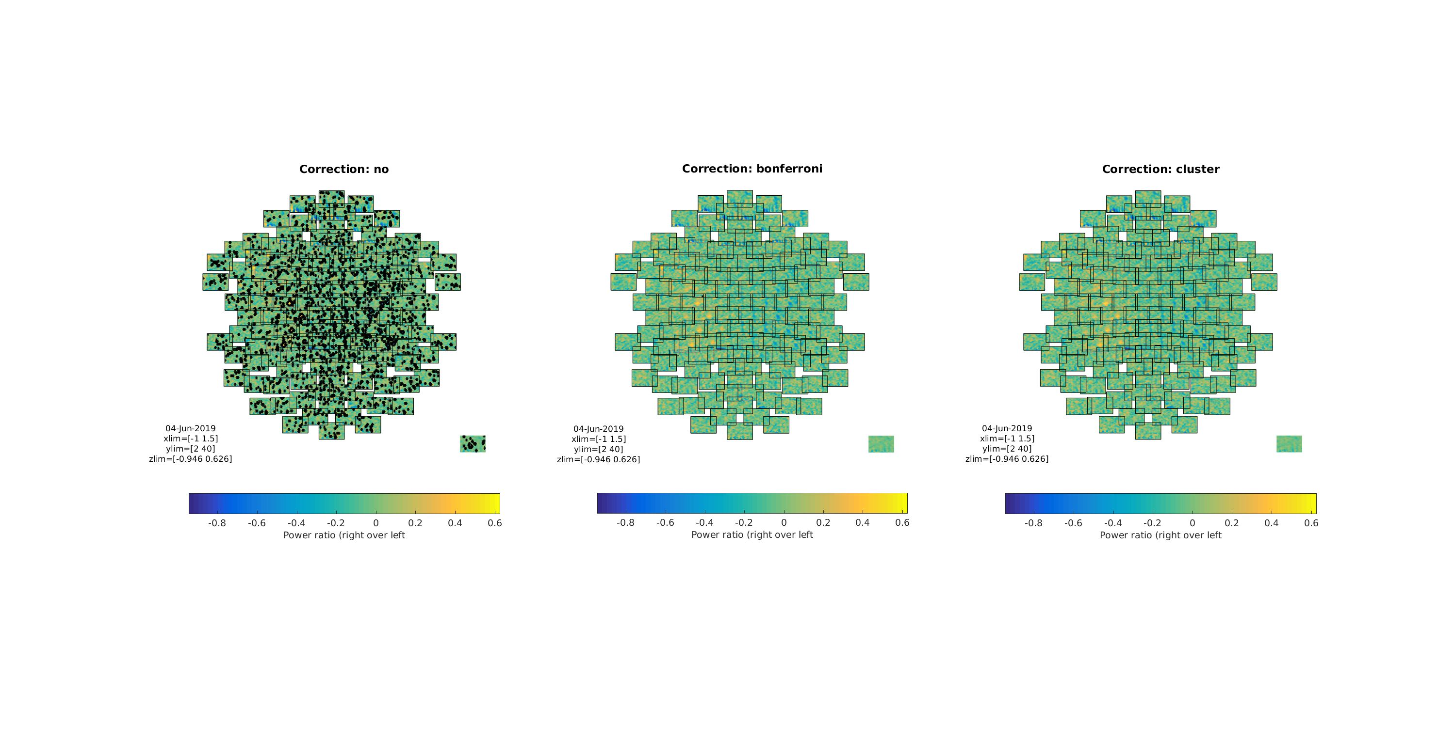
Figure 12: Testing on all frequencies and all latencies Three multiplots showing the differences between the three tests/corrections. Note what this means for the cluster corrected test
Appendix - code snippets for producing images
%% INDICATE EQUIVALENCE (FIG. 4)
figure
subplot(1, 2, 1)
plot(stat_t.time, stat_t.stat(1, :)) % plot t-values for first EEG
title('Stat field for "stat_t"', 'interpreter', 'none')
xlim([stat_t.time(1) stat_t.time(end)])
xlabel('Time (s)')
ylabel('t');

subplot(1, 2, 2)
plot(stat_t_cluster.time, stat_t_cluster.stat(1, :)) % repeat
title('Stat field for "stat_t_cluster"', 'interpreter', 'none')
xlim([stat_t_cluster.time(1) stat_t_cluster.time(end)])
xlabel('Time (s)')
ylabel('t-value');

print -dpng stat_equivalence.png

%% PLOT CLUSTER T-VALUES (FIG. 5)
figure
hold on

plot([stat_t_cluster.posclusters.clusterstat], 'ro')
plot([stat_t_cluster.negclusters.clusterstat], 'bo')
xlabel('Cluster index')
ylabel('T-value')
ylim([-9000 9000])
title('T-values per cluster')
legend({'Positive clusters' 'Negative clusters'})

print -dpng cluster_T_values.png

%% PLOT DISTRIBUTIONS (FIG. 6)

figure('units', 'normalized', 'outerposition', [0 0 0.35 0.5]);
hold on

positive_p = stat_t_cluster.posclusters(1).prob;
negative_p = stat_t_cluster.negclusters(1).prob;

positive_T = stat_t_cluster.posclusters(1).clusterstat;
negative_T = stat_t_cluster.negclusters(1).clusterstat;

positive_text = sprintf(['Observed T\np = ' num2str(round(positive_p, 4))]);
negative_text = sprintf(['Observed T\np = ' num2str(round(negative_p, 4))]);

subplot(1, 2, 1)
histogram(stat_t_cluster.posdistribution, 'facecolor', 'r')
xlabel('Permuted T-values')
ylabel('Observations (#)')
title('Permutation Distribution - Positive')
xlim([0 positive_T + 2500])
ylim([0 60])
arrow([positive_T, 10], [positive_T, 0])
text(positive_T - 2000 , 12, positive_text)

subplot(1, 2, 2)
histogram(stat_t_cluster.negdistribution, 'facecolor', 'b')
xlabel('Permuted T-values')
ylabel('Observations (#)')
title('Permutation Distribution - Negative')
xlim([negative_T - 1000 0])
ylim([0 60])
arrow([negative_T, 10], [negative_T, 0])
text(negative_T - 500 , 12, negative_text)

print -dpng permutation_distributions.png