The purpose of this page is just to serve as todo or scratch pad for the development project and to list and share some ideas.

After making changes to the code and/or documentation, this page should remain on the website as a reminder of what was done and how it was done. However, there is no guarantee that this page is updated in the end to reflect the final state of the project

So chances are that this page is considerably outdated and irrelevant. The notes here might not reflect the current state of the code, and you should not use this as serious documentation.

What is the best way to homogenize data using z-scores?

Z-scores are being used as a means to ‘normalize’ the data before doing over-subjects statistics. However, there are many ways of implementing this and at the moment there is not much consensus what the best method is.

Objectives

to find a proper method for homogenizing data prior to statistical testing, with the purpose of not losing sensitivity (or even possibly gaining sensitivity) in case of a MCP

Step 1: get an overview

what do we want to test (in general terms)
which problems should be solved / why does one need to ‘normalize’ in the first place?
what are the possible solutions?
what are the underlying assumptions?

1. Goal

To homogenize the data on two level

within a dataset (MCP dim)
over datasets (between subjects or repetitions)

What we want to accomplish is at the same time control the false alarm rate, and have max statistical power.

2. Problem

Ad 1)

slow drifts in the data, independent of conditions: this increases variance/reduces the sensitivity (with respect to the effect one is interested in)
different size of effect at different locations and/or frequencies (e.g., 1/f effect in power, or depth bias of beamed power) Ad 2)
large individual differences

3. Possible solution

Ad 1)

baseline correction [to solve slow drifts]
GLM-like solution (regressor for the slow drifts)
multiply with f [to solve 1/f effect]
NAI (neural activity index) [against depth bias of beamed power]

Ad 2)

baseline correction
descriptive statistical measure
ratio between conditions A and B
log(power) [also helps against 1/f effect]
zscores

–> Problem: these solutions may introduce additional noise!

4. Assumption

Properties of the data:

behavior of noise within subjects / trials (stationary or non-stationary)
model of effect (additive or multiplicative)

Step 2: simulate data

The choice of the ‘best’ solution will (probably) depend on the characteristics of the data. Ideally, this will lead to a simple scheme with for each type of data characteristics the optimal method. The choice for the best method for a particular dataset will then depend on the question ‘what are the properties of the data?’.

develop realistic effect and noise models
find optimal noise and effect range

1. Effect and noise model

The simulated dataset should consist of two conditions, baseline and activation, that can be compared and should contain an effect that is small enough to not always be detected by the statistical test. We will ignore the MCP, since cluster randomization effectively deals with that, so it is not of current interest.

The data should be of the for

baseline   = phys           + noise
activation = phys * e1 + e2 + noise

with for the additive effect model: e1 = 1, e2 > 0, and for the multiplicative effect model: e1 > 1, e2 = 0.
phys is the physiological signal, consisting of a ‘constant’ (e.g., alpha oscillation) modulated by a slow drift
noise is the ‘real’ external noise, which is random

phys = phys_constant + phys_noise _ lambda_phys noise = random_noise _ lambda_ext
lambda_phys and lambda_ext are scaling factors for the physiological and external noise, resp.

This gives us the following dimension

effect (for this we will use the ‘freq’ dimension)
noise (for this we will use the ‘time’ dimension)
repetitions (subjects/trials, for this we will use the normal ‘rpt’ dimension)
repetition of the statistical test (for this we will use the ‘chan’ dimension)

This way we can vary the size/range of effect and noise, have multiple trials and at the same time repeat the statistical test several times, using freqstatistics.

2. Find interesting range

We need a range of effect and noise size where at the edges the effect is always found (effect high, noise low) resp. never found (effect low, noise high). In the range in between, it will sometimes turn up, sometimes not. If we repeat the statistical test several times (using the chan dim) and average the results we have a nice measure of the statistical power. Now we can go to the next step and repeat this using the different homogenization methods and see whether they improve the statistical power.

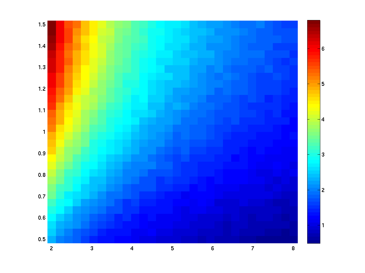
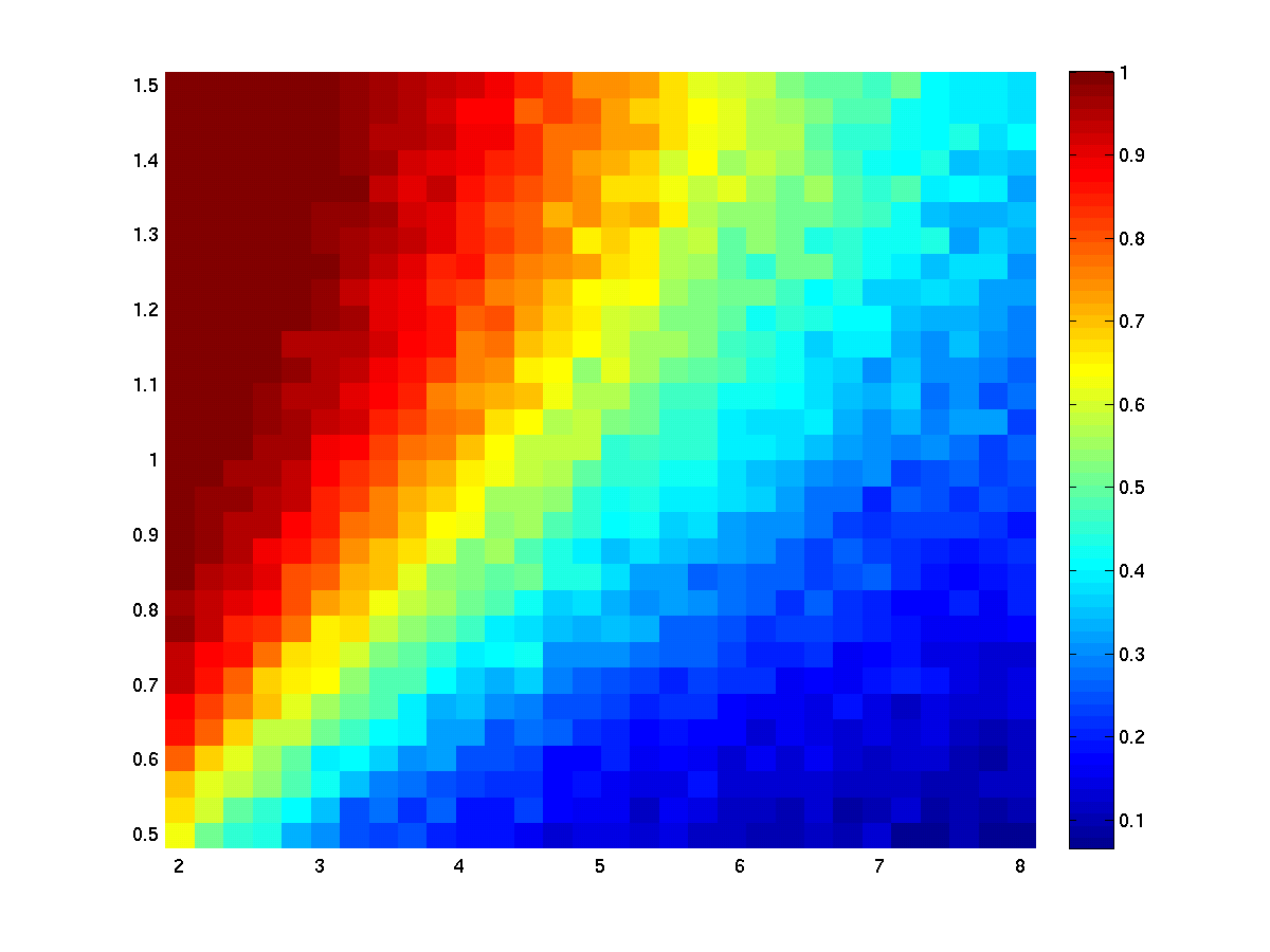
To illustrate (using additive effect model):

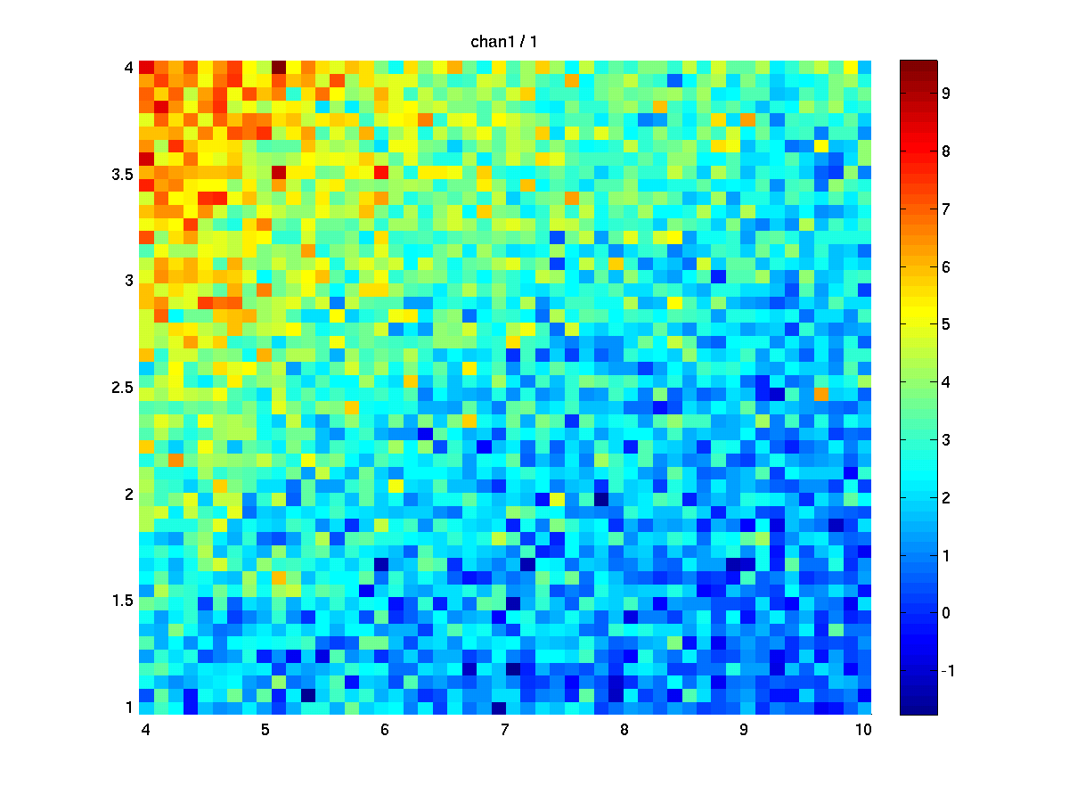
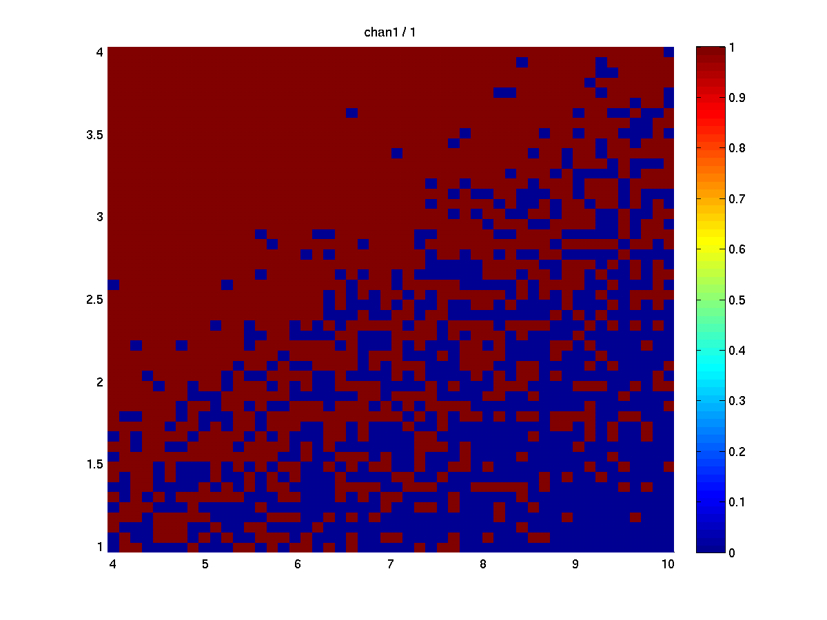
The results of using 1 repetition of the stats test (i.e., 1 channel). The left figure shows ‘stat’, right shows ‘mask’. On the x-axis is noise level, on y-axis effect level, the colouring codes the stat (t values) resp. mask (1=sig effect, 0=no sig effect).

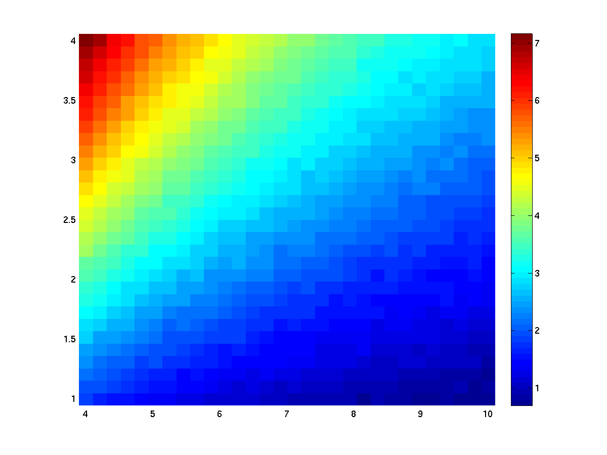
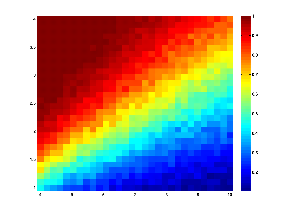
The results of using 500 repetitions of the stats test. Since the noise is randomly generated the results turn out little bit different for each run. Averaging the masks over repetitions reflects the statistical power (=1-beta)