Fit a dipole to the tactile ERF after mechanical stimulation

%%%%%%%%%%%%%%%%%%%%%%%%%%%%%%%%%%%%%%%%%%%%%%%%%%%%%%%%%%%%%%%%%%%%%%%%%%%%
% Tactile Stimulus Dipolefit
%
% In this dataset, mechanical tactile stimuli of 300ms length were applied
% to the right index finger. The tactile stimuli were 5 different patterns
% of which the subject should detect one (deviant: trigger 4). However,
% stimuli were by far too difficult to differentiate, so they can be pooled
% across all of them. There are no button presses or anything else in the
% data. Because stimuli were too difficult there was absolutely no task.
%
% The MEG dataset is available from
%   https://download.fieldtriptoolbox.org/tutorial/SubjectBraille.zip
%
%%%%%%%%%%%%%%%%%%%%%%%%%%%%%%%%%%%%%%%%%%%%%%%%%%%%%%%%%%%%%%%%%%%%%%%%%%%%

% determine interesting segments in the data

cfg                     = [];
cfg.dataset             = 'SubjectBraille.ds';
cfg.continuous          = 'yes';
cfg.trialdef.eventtype  = 'backpanel trigger';
cfg.trialdef.eventvalue = [4,8];
cfg.trialdef.prestim    = 0.4;
cfg.trialdef.poststim   = 0.6;
cfg = ft_definetrial(cfg);

% remove the first and last 10 trials: they are too close to the edge
% of the file, which causes problems with the 10 seconds filter padding
cfg.trl = cfg.trl(10:(end-10),:);

% the following settings are relevant for later preprocessing, but can be
% specified already. The artifact detection routines will adjust their
% default settings according to the specified filter padding.
cfg.padding           = 10;        % for filtering
cfg.dftfilter         = 'yes';     % line noise removal
cfg.demean            = 'yes';     % baseline correction
cfg.baselinewindow    = [-inf 0];  % use the pre-trigger interval
cfg.channel           = 'MEG';     % only read in the MEG channels

%%%%%%%%%%%%%%%%%%%%%%%%%%%%%%%%%%%%%%%%%%%%%%%%%%%%%%%%%%%%%%%%%%%%%%%%%%%%
% detect squid jump artifacts
% this artifact detection takes very long, since it has to be done on all 151 MEG channels
% since the data does not contain SQUID jump artifacts, this step can be skipped
% cfg.artfctdef.jump.sgn       = {'MEG'};
% cfg = ft_artifact_jump(cfg);

%%%%%%%%%%%%%%%%%%%%%%%%%%%%%%%%%%%%%%%%%%%%%%%%%%%%%%%%%%%%%%%%%%%%%%%%%%%%
% detect eye artifacts
% use only defaults
cfg.artfctdef.eog.sgn         = 'EOG'; % {'MLT21' 'MRT21' 'MLT31' 'MRT31' 'MLF12' 'MRF12'};
cfg.artfctdef.eog.feedback    = 'yes';
cfg = ft_artifact_eog(cfg);

%%%%%%%%%%%%%%%%%%%%%%%%%%%%%%%%%%%%%%%%%%%%%%%%%%%%%%%%%%%%%%%%%%%%%%%%%%%%
% detect muscle artifacts
% the temporal and the occipital channels pick up most of the muscle activity
cfg.artfctdef.muscle.sgn      = {'MLT' 'MRT'} % 'MRO' 'MLO'};
cfg.artfctdef.muscle.feedback = 'yes';
cfg.artfctdef.muscle.cutoff   = 40;  % has been determined by visual inspection
cfg = ft_artifact_muscle(cfg);

%%%%%%%%%%%%%%%%%%%%%%%%%%%%%%%%%%%%%%%%%%%%%%%%%%%%%%%%%%%%%%%%%%%%%%%%%%%%
% artifact removal and preprocessing
%
% after detecting the segments of data contaminated by artifacts, those
% segments subsequently are removed and the clean data segments of interest
% can finally be imported into MATLAB using the ft_preprocessing function.
cfg.artfctdef.minaccepttim    = 0.2;
cfg.artfctdef.reject          = 'partial';
cfg.artfctdef.feedback        = 'yes';
cfg = ft_rejectartifact(cfg);

% read and preprocess the data
data = ft_preprocessing(cfg);

%%%%%%%%%%%%%%%%%%%%%%%%%%%%%%%%%%%%%%%%%%%%%%%%%%%%%%%%%%%%%%%%%%%%%%%%%%%%
% compute the ERF
cfg = [];
cfg.channel = 'MEG';
cfg.vartrllength = 2;
avg = ft_timelockanalysis(cfg, data);

%%%%%%%%%%%%%%%%%%%%%%%%%%%%%%%%%%%%%%%%%%%%%%%%%%%%%%%%%%%%%%%%%%%%%%%%%%%%
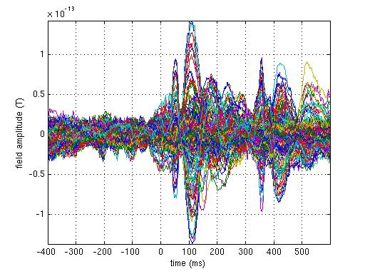
% make a butterfly plot of the ERF
% using the plain MATLAB plotting function
figure
plot(1000*avg.time, avg.avg)  % convert time to ms
xlabel('time (ms)')
ylabel('field amplitude (T)')
axis tight
grid on

%%%%%%%%%%%%%%%%%%%%%%%%%%%%%%%%%%%%%%%%%%%%%%%%%%%%%%%%%%%%%%%%%%%%%%%%%%%%
% make a topographic plot of the ERF, in steps of 5ms
cfg = [];
cfg.xlim = 0:0.005:0.1;
cfg.colorbar = 'no';
cfg.comment = '';
cfg.showxlim = 'no';
cfg.showzlim = 'no';
cfg.zlim = [-1.5 1.5] * 1e-13;
figure
ft_topoplotER(cfg, avg);

%%%%%%%%%%%%%%%%%%%%%%%%%%%%%%%%%%%%%%%%%%%%%%%%%%%%%%%%%%%%%%%%%%%%%%%%%%%%
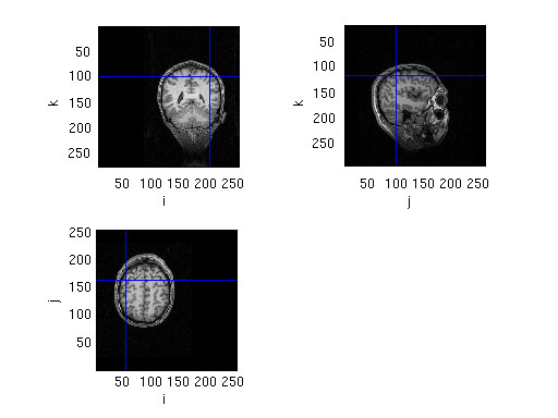
% fit a dipole to the M50 and M100 components
cfg = [];
cfg.latency = [0.045 0.055];  % specify latency window around M50 peak
cfg.numdipoles = 1;
cfg.hdmfile = 'SubjectBraille.hdm';
cfg.feedback = 'textbar';
cfg.resolution = 2;
cfg.unit = 'cm';
dipM50 = ft_dipolefitting(cfg, avg);
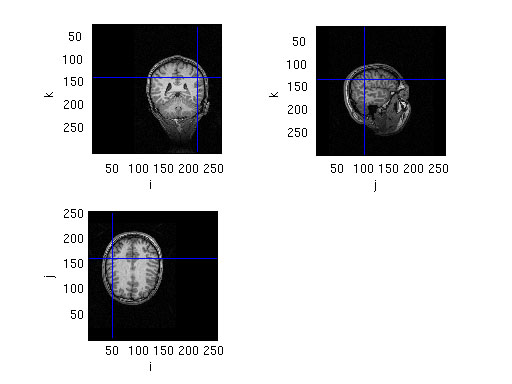
cfg.latency = [0.100 0.120]; % specify latency window around M100 peak
dipM100 = ft_dipolefitting(cfg, avg);

%%%%%%%%%%%%%%%%%%%%%%%%%%%%%%%%%%%%%%%%%%%%%%%%%%%%%%%%%%%%%%%%%%%%%%%%%%%%
% make a plot of the location of the dipoles
% read the anatomical MRI
mri = ft_read_mri('SubjectBraille.mri');

% the source is expressed in cm, the MRI is expressed in mm
cfg = [];
cfg.location = dipM50.dip.pos * 10;   % convert from cm to mm
figure; ft_sourceplot(cfg, mri)
cfg.location = dipM100.dip.pos * 10;  % convert from cm to mm
figure; ft_sourceplot(cfg, mri)