Using simulations to estimate the sample size for cluster-based permutation test
This example is contributed by Dr. Cheng Wang.
It is recommended and sometimes even required to provide justification for sample size prior to starting a study and when reporting about it (Clayson et al., 2019). Many researchers use G*Power to estimate the sample size required for their studies. However, although very useful and popular, this software is not suitable for multivariate data or for non-parametric tests. For EEG and MEG we often use a cluster-based permutation test, which is a non-parametric test that exploits the multivariate structure in the data.
Here, we demonstrate two easy-to-use MATLAB functions that use simulations to estimate the sample size for cluster-based permutation tests. These functions can be used for EEG/MEG research involving t-test between two conditions, one-way ANOVA with three or more conditions, or 2xN interactions. The experiment can be of a with-subjects, between-subjects, or mixed design. The functions were written for, and first used in Wang and Zhang (2021). Please cite this paper where appropriate.
From this OSF project, you can download the functions and the corresponding demo files. The MATLAB functions are stored in the functions folder.
- sampleSize_erp.m is for ERP data
- sampleSize_timefreq.m is for time-frequency data
Two demo files demonstrating how to use the functions are in the demo folder:
- demo_erp.m
- demo_timefreq.m
In this example, we will first briefly introduce how to estimate sample size through simulations using an intuitive example of coin-tossing. Then, we will demonstrate how to estimate sample size through simulations for t-tests and cluster-based permutation tests.
Power analysis through simulations – an intuitive example of coin-toss
Let’s start by a brief introduction to estimate sample size using an intuitive example of coin-tossing. For a more detailed and excellent introduction, please see Dr. Julian Quandt’s website. The following section is inspired by Dr. Quandt’s excellent introduction.
Suppose we are presented with a coin and we want to know whether it is fair (50% chance lands on head). We can test it by running coin-tossing experiments. Consider the following two experiment scenarios. In Experiment 1, we tossed it 2 times, and observed 2 heads; In Experiment 2, we tossed it 5 times and observed 5 heads. With either experiment, we are inclined to think the coin is unfair. But intuitively, we will be more confident of the coin’s unfairness following Experiment 2 than following Experiment 1. But still, we don’t know how sure we are about our decision to call the coin unfair. We can clarify this using inferential statistics.
- Null hypothesis H0: the coin is fair, i.e., 50% chance for heads and 50% chance for tails
- Alternative hypothesis H1: the coin is totally unfair, e.g., 100% chance to land on head
- Sample size: 2 or 5 samples (tosses)
- Power: the probability of rejecting the null hypothesis when H0 is false
The power of a statistical test quantifies how sure we can be to decide the coin is unfair (i.e., rejecting the null hypothesis). By definition, we can calculate power by doing the same experiment a large number of times (e.g., 5000 times), and then calculating the proportion of the number of times in which null hypothesis can be rejected to 5000. However, even a simple task such as coin-tossing will be very time-consuming and tedious when you need to repeat it 5000 times. Luckily, we don’t really have to toss a coin, as MATLAB can simulate the results for us. We know the outcome of tossing a coin conforms to a binomial distribution. Using this distribution, we can simulate the outcome of each experiment (i.e., the number of heads out of a certain number of tosses).
First, we need to “guess”, based usually on pilot studies or prior similar studies, the key parameters of the binomial distributions for each of the null and alternative hypotheses. In the current example, the chance of a coin to land on head under the null hypothesis is undoubtedly 50%. And under the alternative hypothesis, we will assume that the coin has a chance of 100% to land on head, based on the result our observations so far. Only with these parameters specified can data be sampled from the distributions. Note that the difference (50% vs. 100%) between the two hypotheses can be construed as the effect size, which has great influence on power: statistical power tends to be greater with larger effect size.
Once you are done with this example, you may want to continue reading this example on estimating and reporting the effect size following a cluster-based test.
Second, we need to decide the criterion for rejecting the null hypothesis. Conventionally, we reject the null hypothesis if the probability of its being correct is less than 0.05 or 5%, which is the so-called alpha level. In each experiment, if the outcome is unlikely (i.e., the probability < 0.05) to happen under the null hypothesis, we reject the null hypothesis.
Finally, power is calculated as the proportion of the null hypothesis being rejected following a very large number (say 5000) of repetitions of the experiment. Take the current case for example, the outcome of tossing a 100% unfair coin 5 times can be sampled from the binomial distribution, and the results would always be 5 heads. The probability of 5 heads out of 5 tosses under the null hypothesis is 1/(2^5) = 0.0313 < 0.05. So, in all of the 5000 experiments, the null hypothesis is rejected. Thus, the power is 1 = 5000/5000.
All of the above steps can be done using the following block of MATLAB code:
% settings
p_heads_h1  = 1;     % chance to land on head under H1, aka, the effect size
n_sample    = 5;     % sample size, i.e., number of toss
alpha_level = 0.05;  % alpha level
n_sim       = 5000;  % number of simulations/experiments

% run 5000 experiments of tossing a 100% unfair coin 5 times, store the number of heads generated in each experiment
n_heads = binornd(n_sample, p_heads_h1, [1,n_sim]);
% calculate the probability of getting at least that many heads if the coin would be fair
p_h0  = 1-binocdf(n_heads -1, n_sample, 0.5);
% calculate power
power = sum(p_h0 < alpha_level)/n_sim
A 100% unfair coin is an extreme and simplified example. You can try other settings in the above MATLAB code and see what you get. For example, if we estimate that the coin has a chance of 55% to land on head, and the sample size is 100, we can estimate the power to be 0.241, which is close to the result from G*Power.
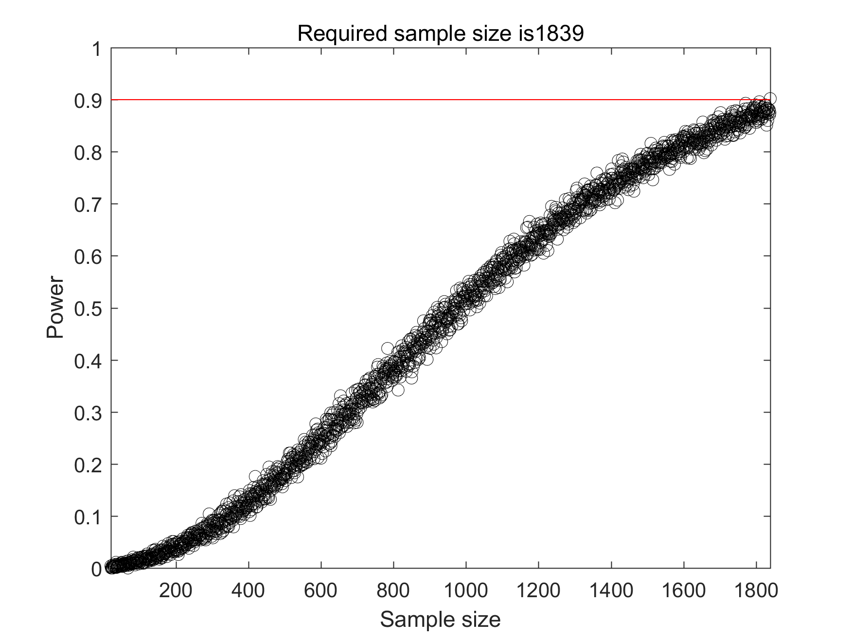
The previous code only shows how to calculate power with a specified sample size through simulation. The following code will show how to estimate the required sample size for a desired power (e.g., 0.9). Basically, what the code does is calculating the power through simulations for each sample size, starting from 21, increasing in steps of 1, until it reaches a power of 0.90. The code will stop when the power reaches the desired level, and the sample size corresponding to this desired power is the sample size we need for this test.
% settings
alpha_level = 0.001;   % alpha level
power_level = 0.9;     % desired power level
p_heads_h1  = 0.55;    % chance to land on head under H1
n_start     = 20;      % sample size to start
n_sim       = 1000;    % number of experiments

% run simulations for each sample size until power reaches desired level
power      = 0;                  % initialize the variable
power_at_n = zeros(1,n_start);   % initialize
n_sample   = n_start;            % sample size
while power < power_level        % continue increasing sample-size until power reach desired level
    n_sample = n_sample + 1;     % sample size in current iteration
    disp(n_sample);
    n_heads = binornd(n_sample, p_heads_h1, [1,n_sim]);
    p_h0  = 1-binocdf(n_heads-1, n_sample, 0.5);
    power = sum(p_h0 < alpha_level)/n_sim;  % calculate power for the current sample size
    power_at_n(n_sample) = power;
end

% plot the result
plot(1:n_sample, power_at_n, 'ko'); hold on
plot([0 n_sample],[power_level power_level],'r');
xlim([n_start+1 n_sample]); ylim([0 1])
xlabel('Sample size'); ylabel('Power')
title(['Required sample size is' num2str(n_sample)])
From the above example, we can summarize the basic steps to estimate sample size through simulation:
- Specify a null hypothesis, an alpha-level, and a desired power,
- Specify an alternative hypothesis, which is per se a theoretical distribution from which data can be sampled or simulated. This will also determine the effect size.
- Start from a small sample size. simulate data 1000 times from the distribution with this sample size. In each time, estimate the probability of the simulated data happening under the null hypothesis. If the probability is less than the alpha level, reject the null hypothesis. Then calculate power as the proportion of the number of times rejecting null hypothesis to 1000.
- Continue increasing the sample size until the power reaches the desired level.
Estimating sample size through simulations – t-test
A more realistic problem that we encounter in our daily research life is comparing two conditions. Suppose we have two conditions of (independent) data, how can we estimate the required sample size through simulations? We can do it following the above four steps.
- Null hypothesis H0: no difference between the two conditions; for instance, alpha = 0.05; desired power = 0.8.
- Alternative hypothesis H1: significant difference between the two conditions. The key is to define the two normal distributions from which the two groups of data can be sampled. So, the means and standard deviations need to be specified for each of the two conditions, based on prior existing or pilot studies. Usually, the standard deviations are assumed to be equal, whereas the means are different. The distance between the two means relative to the standard deviation reflects the effect size.
- Starting from a small sample size, we use the theoretical distribution to simulate two groups of data 1000 times. Each time, we estimate the significance (i.e., p values) of the difference between the two conditions using a t-test. If probability < 0.05, we reject the null hypothesis. Then, calculate power as the proportion of the number of times that the null hypothesis is rejected.
- Continue increasing the sample size until the power reaches the desired level.
The following block of MATLAB code implements these steps.
% settings
alpha_level = 0.05;      % alpha level
power_level = 0.80;      % desired power level
mu          = [3 4];     % means for the two conditions
sd          = [2 2];     % standard deviations for the two conditions
n_start     = 10;        % sample size to start
n_sim       = 1000;      % number of experiment

% run simulations for each sample size until power reaches desired level
power      = 0;                  % initialize the variable
power_at_n = zeros(1,n_start);   % initialize
n_sample   = n_start;            % sample size
while power < power_level  % continue increasing sample-size until power reach desired level
    n_sample = n_sample + 1;   % sample size in current iteration
    p_vals   = ones(1,n_sim);  % initialize
    for i=1:n_sim
        rd1 = normrnd(mu(1), sd(1), n_sample, 1);  % sampling data from a normal distribution for group1
        rd2 = normrnd(mu(2), sd(2), n_sample, 1);  % sampling data from a normal distribution for group2
        [~,p_vals(i),~,~] = ttest2(rd1,rd2);  % t-test, store the p values
    end
    power = sum(p_vals < alpha_level)/n_sim;  % calculate power for the current sample size
    power_at_n(n_sample) = power;
end

% plot the result
figure
plot(1:n_sample, power_at_n, 'ko'); hold on
plot([0 n_sample],[power_level power_level],'r'); ylim([0 1])
xlim([n_start+1 n_sample]); ylim([0 1])
xlabel('Sample size'); ylabel('Power')
title(['Required sample size is ' num2str(n_sample)])
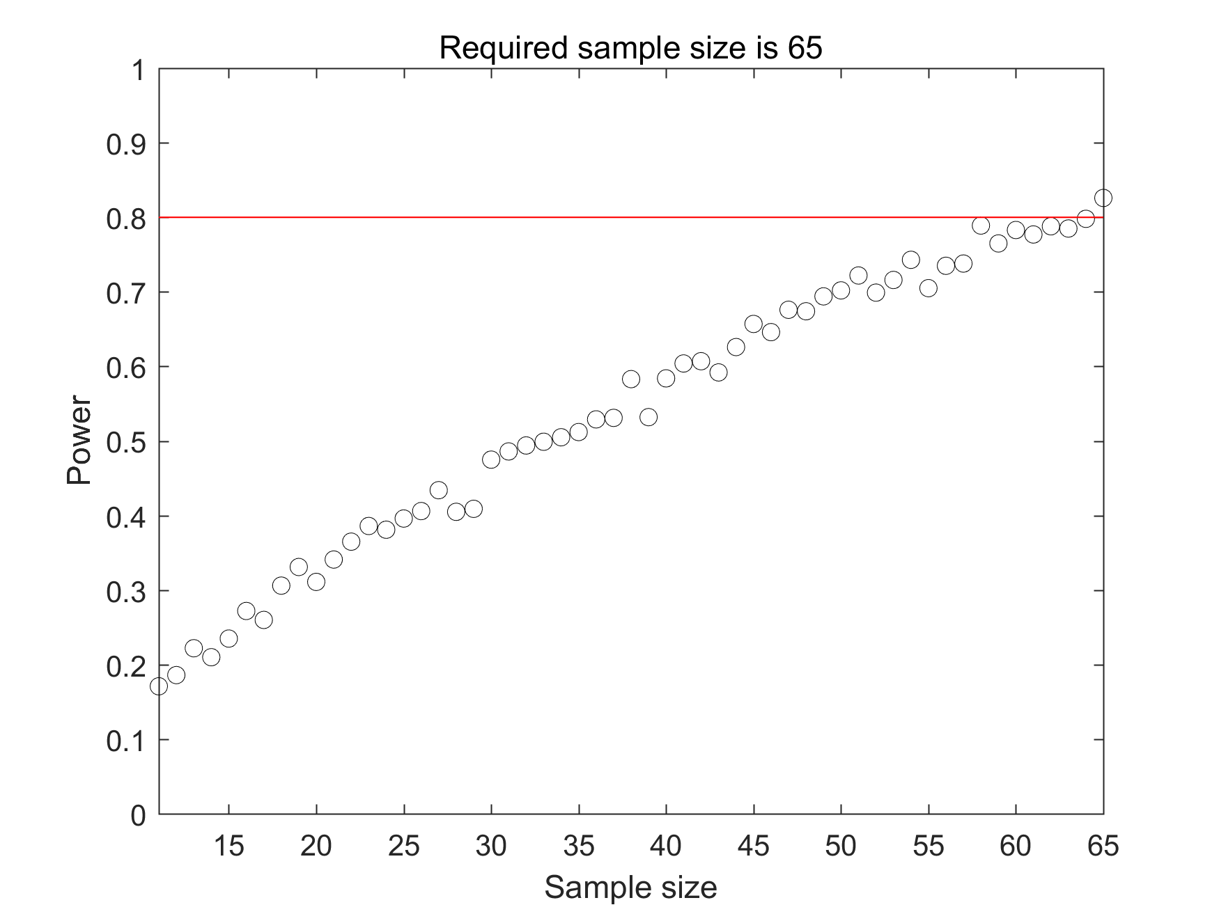
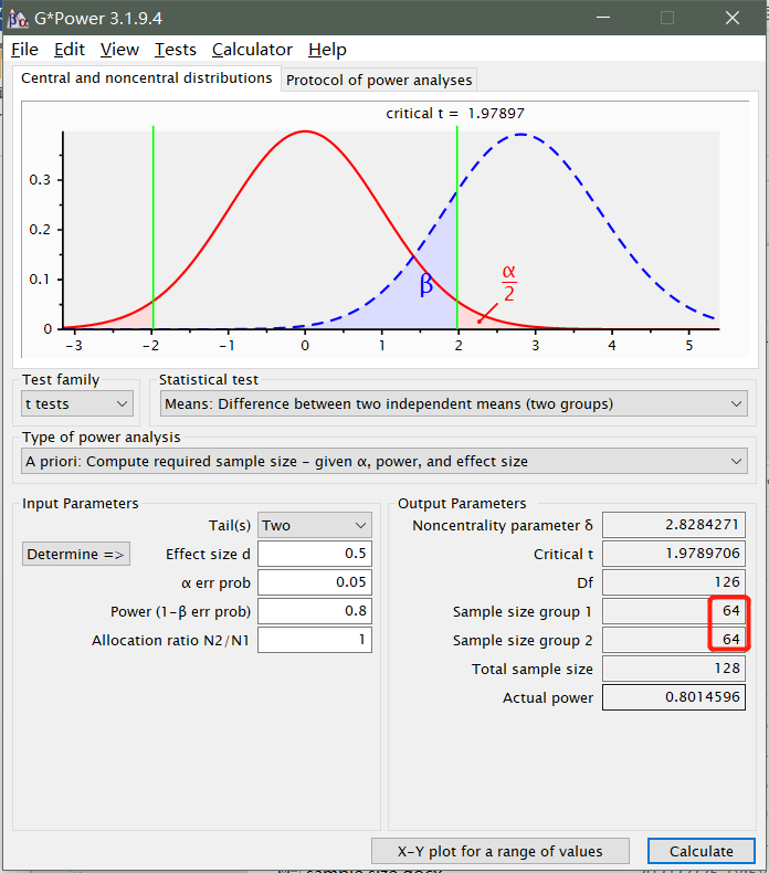
The result shows that the sample size required for 80% power in an independent t-test (means: 3 vs. 4; SDs = 2) is 65, which is very close to the result that we can obtain from G*Power.
Estimating sample size through simulations - cluster-based permutation test
For cluster-based permutation tests in MEG/EEG data, the method of estimating sample size through simulations is the same to that for t-tests, except that Step 3 is somewhat different. In the Step 3 for cluster-based permutation tests, several groups of ERP (2 dimensions: channelxtime) or time-frequency (3 dimensions: channelxfrequencyxtime) data are simulated. In each sample of the ERP/time-frequency data, we simulate a cluster of interest with a predefined time window (e.g., 50-250 ms) and frequency band (e.g., 4-8 Hz) in neighboring channels (e.g., C1, CZ, CP1, CPZ). The time, frequency, and spatial ranges of the cluster can be chosen to be similar to those of cluster displaying effect of interest in your pilot studies or prior existing studies. The cluster’s peak values in the two conditions were sampled from two normal distributions (for a between-subject design) or a bivariate normal distribution (for a within-subject design). The means and standard deviations of the distributions can be chosen to be similar to those in prior existing or pilot studies.
Then a cluster-based permutation test is performed on the simulated dataset to test whether there is a significant difference between the two conditions. We run the simulations for 1000 times, and the power is calculated as the proportion of the number of times that the null hypothesis is rejected. These simulations can subsequently be repeated for an incrementally increasing sample size, starting from 10, increasing in steps of 1, until the power reached the desired threshold (e.g., 0.8). The above processing is implemented in the two aforementioned MATLAB functions sampleSize_erp.m and sampleSize_timefreq.m.
Next, we will demonstrate how to use the sampleSize_timefreq.m function; the usage of sampleSize_erp.m is very similar. See also the two demo files.
First, you need to have a time-frequency dataset that is generated by the ft_freqanalysis function. You can also use the exempleData_timefreq.mat dataset which can be downloaded with the functions from OSF. This dataset is used only for retrieving the data structure for simulating time-frequency data. The sampleSize_timefreq.m function has two parts of parameters, which are respectively stored in cfg and stat_cfg. The structure cfg stores the configurations for simulating the data, and stat_cfg stores the configurations for the cluster-based permutation tests.
%%
clear; close all;
addpath('F:\SampleSize\functions')
load('exampleData_timefreq.mat');   % load a time-freq data obtained from the ft_freqanalysis function,
                                    % to retrieve the fieldtrip data structure

%=========== set configuration for data simulation ================
% parameters for the power analysis
cfg = [];
cfg.alpha_level = 0.05;    % desired alpha-level
cfg.power_level = 0.8;     % desired power
cfg.num_sims    = 500;     % number of randomizations, should be >= 500
cfg.n_start     = 10;      % sample size to start with, should be <=10

% parameters for normal distribution from which the simulated data are sampled
cfg.ExpDesign   = 'within-subjects';  % 'within-subjects' or 'between-subjects'
cfg.mu          = [5 3];   % mean of each condition. Can have two or more conditions, the function will automatically select
                           % a t-test for two conditions, and a F-test for three or more conditions for the cluster-based permutation test
cfg.sd          = [2 2];   % standard deviation of each condition
cfg.cor         = 0.7;     % minimum correlation between paried samples, ONLY needed for a within-subject design
% mu, sd, and cor should be corresponding values that you expect from your own data, they can be set to be similar to those in pilot or prior existing studies
% mu is particularly important, as it determines the amount of difference between conditions

% parameters for the time-freq data, should be matched to your own time-freq data
cfg.time           = exampleData.time;   % exampleData is the variable loaded from 'exampleData_timefreq.mat'
cfg.freq           = exampleData.freq;
cfg.label          = exampleData.label;
cfg.dimord         = exampleData.dimord;

% parameters for the simulated cluster of interest
% these three parameters should be set similar to those of the cluster in pilot or prior existing studies
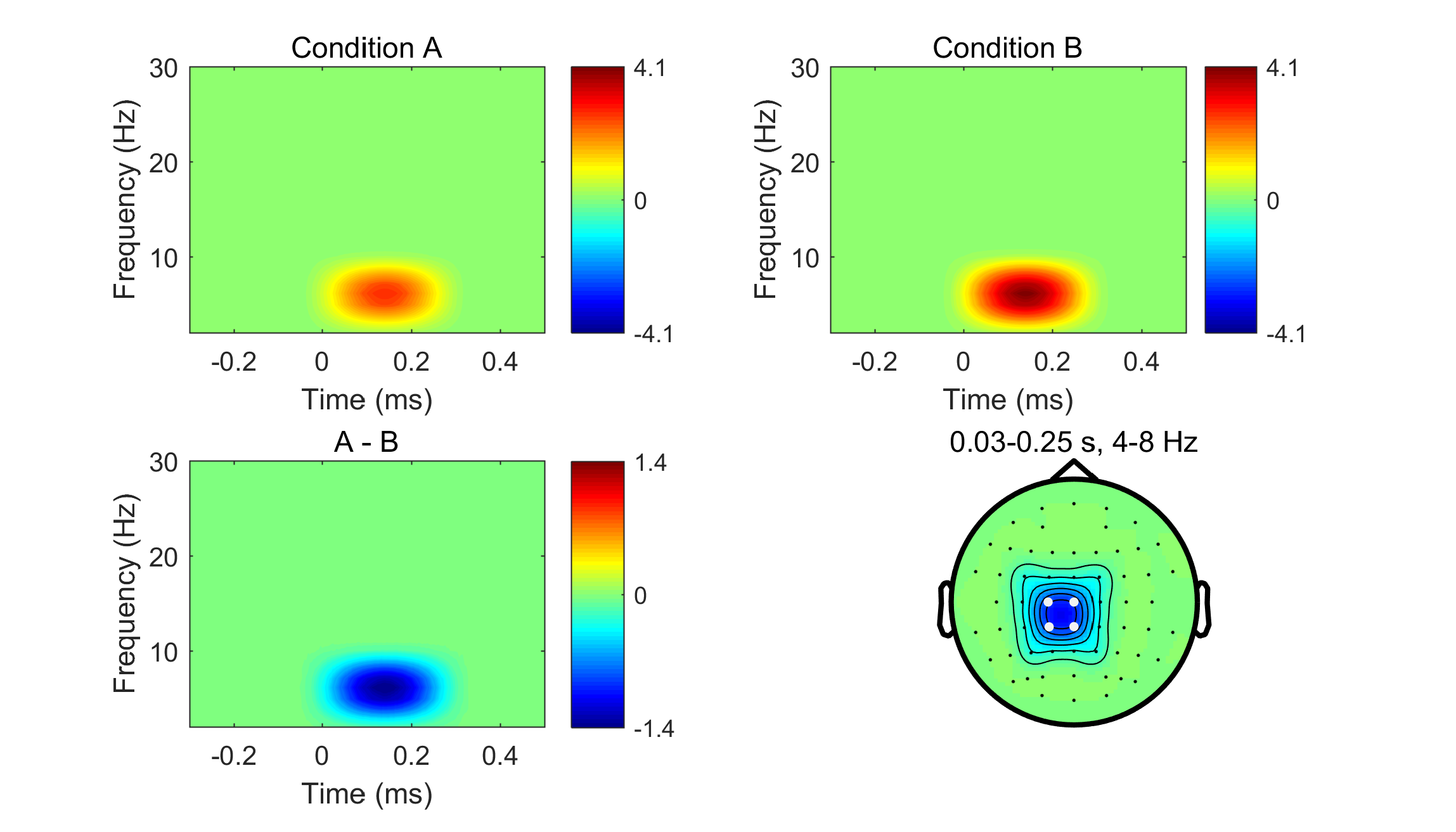
cfg.clusterfreq    = [4 8];                    % freq range you want to be included in the cluster displaying effect of interest,
cfg.clustertime    = [0.03 0.25];              % time range you want to be included in the cluster displaying effect of interest,
cfg.clusterchan    = {'CZ','C1','CPZ','CP1'};  % channles you want to be included in the cluster displaying effect of interest

% channels surrounding the cluster channels, used as a buffer zone from peak values in the cluster channels to 0
cfg.bufferchan     = {'FC3','FC1','FCZ','FC2','C2','CP2','P2','PZ','P1','P3','CP3','C3'};
cfg.layout         = 'NeuroScan_quickcap64_layout.lay';  % your layout file

%=========== set configuration for cluster permutation test ================
neighbour_cfg = [];
neighbour_cfg.method      = 'triangulation';
neighbour_cfg.layout      = cfg.layout;
neighbour_cfg.feedback    = 'no';
neighbours = ft_prepare_neighbours(neighbour_cfg, exampleData);

stat_cfg = [];
stat_cfg.neighbours       = neighbours;
stat_cfg.minnbchan        = 3;
stat_cfg.channel          = {'all','-HEOG','-VEOG'};
stat_cfg.avgoverchan      = 'no';
stat_cfg.latency          = [0 0.5];     % in second
stat_cfg.avgovertime      = 'no';
stat_cfg.frequency        = 'all';
stat_cfg.avgoverfreq      = 'no';
stat_cfg.method           = 'montecarlo';
stat_cfg.correctm         = 'cluster';
stat_cfg.clusterstatistic = 'maxsum';   % 'maxsum' or 'maxsize'
stat_cfg.clustertail      = 0;          % 0 for t-test (two tails); 1 for F test (right tail)
stat_cfg.clusteralpha     = 0.05;
stat_cfg.tail             = 0;          % 0 for t-test (two tails); 1 for F test (right tail)
stat_cfg.alpha            = 0.05;
stat_cfg.numrandomization = 500;        % number of randomizations, should be >= 500

%%% Run the function
MyPar = parpool; % start parallel pool
res = sampleSize_timefreq(cfg,stat_cfg);
save('results_timefreq_pairedSamples.mat','res')
delete(MyPar)
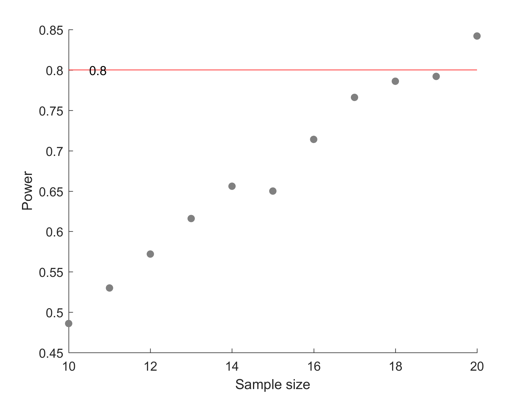
Running this function would be quite time-consuming, with a lot of simulations to run. It can therefore be time-saving to open parpool to use parallel computing. The results are stored in res. The following block of code plots the results.
%% plot the results of power analysis
cfg = res.cfg;
figure
scatter(cfg.n_start:res.sample_size, res.power_at_n(cfg.n_start:end),400,[0.5 0.5 0.5],'Marker','.'); hold on
plot([cfg.n_start res.sample_size],[cfg.power_level cfg.power_level], 'r')
text(cfg.n_start+0.5, 0.8,'0.8')
xlabel('Sample size'); ylabel('Power'),xlim([cfg.n_start res.sample_size])
We can also have a look at the simulated data for the required sample size. The datasets for the two conditions are stored in res.condA and res.condB.
% compute the grand average
cfg1 = [];
cfg1.channel   = 'all';
cfg1.toilim    = 'all';
cfg1.foilim    = 'all';
for ci=1:length(cfg.mu)
    grand = ft_freqgrandaverage(cfg1, res.allsub{ci}{:});  % grand-avg
    clusterchan_idx = match_str(cfg.label,cfg.clusterchan);
    pow(ci,:,:)     = squeeze(mean(grand.powspctrm(clusterchan_idx,:,:),1));    % average cross cluster channels
end

figure
lim = round(max(abs(pow(:))),1);
nrow = ceil(sqrt(length(cfg.mu)));
for ci=1:length(cfg.mu)
    subplot(nrow,nrow,ci)
    contourf(cfg.time, cfg.freq, squeeze(pow(ci,:,:)), 40, 'linecolor','none')
    set(gca, 'clim', [-lim lim]); colorbar; colormap(jet);
    xlabel('Time (ms)'); ylabel('Frequency (Hz)')
    colorbar('YTick', [-lim 0 lim]);
end
Testing interactions
The two functions can also be used to estimate the sample size for 2-by-N (N>=2) interaction effect, however, the first factor must be a within-subjects factor and the second can be a within- or between-subjects factor.
Take a 2x3 design for example, the first and second factors can be respectively denoted A and B, and the six cells in this design can be denoted A1B1, A2B1, A1B2, A2B2, A1B3 and A2B3. For each subject, we can compute the difference between the two levels of A, denoted as A1B1minusA2B1, A1B2minusA2B2, and A1B3minusA2B3. Now testing an interaction effect between A and B can be treated as comparing these three difference scores, which can be done by a one-way ANOVA using ft_statfun_depsamplesFmultivariate if B is a within-subjects factor, or ft_statfun_indepsamplesF if B is a between-subjects factor. If B has only two levels, you can simply use a t-test to compare the two differences (i.e., A1B1minusA2B1 and A1B2minusA2B2). Uing this approach, we can test an interaction effect using cluster-based permutation test. See this page for more details.
Thus, we can treat two-way ANOVA as comparing differences by using t-tests or one-way ANOVAs. As to the configuration of the functions, simply enter the means, standard deviations, and correlations of these differences you expect for your data respectively into the cfg.mu, cfg.sd, and cfg.cor fields in the demo m-files.
See also
- https://osf.io/rmqhc
- https://www.psychologie.hhu.de/arbeitsgruppen/allgemeine-psychologie-und-arbeitspsychologie/gpower.html
- Example script for estimating and reporting the effect size following a cluster-based test
- Other pages on this website that are tagged with statistics
