Getting started with QuSpin OPM data

QuSpin is based in Louisville, Colorado, USA, and develops miniature, optically-pumped magnetometer (OPM) sensors for functional brain imaging and other applications. The QuSpin magnetometer sensors are used in their own MEG systems, but also in the MEG systems from Cerca Magnetics. Here we will be discussing only the QuSpin MEG system itself.

File formats

The QuSpin acquisition software records the raw data in the .lvm format, which can be converted into the .fif format for further processing.

The data used in this example is available from our download server.

Data in the .lvm format

The .lvm files are ASCII text files with a header, followed by a tabular section with the data for each channel and sample. The .lvm files do not contain information on the location and orientation of the sensors. Reading these large ASCII files is relatively inefficient, hence we recommend to read them as continuous data into memory in one go, and then segment them.

cfg = [];
cfg.dataset = 'VEP-raw.lvm';
data_continuous = ft_preprocessing(cfg);

cfg = [];
cfg.channel = 'Z*';
cfg.blocksize = 30; % seconds
ft_databrowser()

We have to read the file once more to parse the events in the trigger channels. We use ft_definetrial for this, which uses a trial function to select events and define segments around them as trials to be further processed.

cfg = [];
cfg.dataset = 'VEP-raw.lvm';
cfg.trialfun = 'ft_trialfun_general';
cfg.trialdef.prestim = 0.1;
cfg.trialdef.poststim = 0.5;
cfg.trialdef.eventtype = 'D1';
cfg = ft_definetrial(cfg);
trl = cfg.trl;

Using the trial definition trl, we can cut the segments of interest.

cfg = [];
cfg.trl = trl;
data_segmented = ft_redefinetrial(cfg, data_continuous);

cfg = [];
cfg.baselinewindow = [-inf 0];
cfg.demean = 'yes';
data_segmented = ft_preprocessing(cfg, data_segmented);

These can be averaged and plotted.

cfg = [];
timelock = ft_timelockanalysis(cfg, data_segmented);

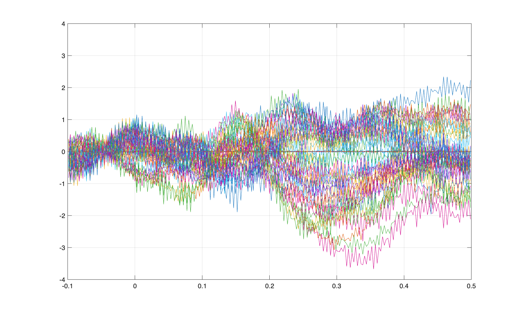
figure
sel = startsWith(timelock.label, 'Z');
plot(timelock.time, timelock.avg(sel,:));
ylim([-4 4])
grid on

Data in the .fif format

The initial data is recorded in the .lvm format, and can be converted to the generic .fif format using scripts provided by QuSpin. In this conversion process the sensor information can be added, either by the sensor positions and orientations being known - given the 3D printed helmet that was used during recording - or using the HALO system.

Processing the data in .fif format is not so different from the .lvm format, except that the data is much faster to read and that triggers or events are represented slightly differently.

cfg = [];
cfg.dataset = 'VEP-raw.fif';
cfg.lpfilter = 'yes';
cfg.lpfreq = 40;
cfg.hpfilter = 'yes';
cfg.hpfreq = 0.5;
cfg.channel = {'X*', 'Y*', 'Z*'};
data_continuous = ft_preprocessing(cfg);

Not all channels that are present in the file were actually connected to a sensor and recorded, so some channels don’t contain any signal. We can select the working channels by looking at which channels have a position (which was determined using the HALO procedure).

sel = find(isnan(data_continuous.grad.coilpos(:,1)));
badchannel = data_continuous.grad.label(sel);

cfg = [];
cfg.channel = setdiff(data_continuous.label, badchannel);
data_continuous = ft_selectdata(cfg, data_continuous);

We can look at channels that have a lot of variance, which we can remove from the subsequent analysis.

cfg = [];
cfg.method = 'summary';
cfg.mychan = data_continuous.label;
cfg.chanscale = 1e15;
ft_rejectvisual(cfg, data_continuous);

badchannel = {
    'X45',
    'Y17',
    'Y36',
    'Y45',
    'Y47',
    'Y48',
    'Y49',
    'Z28',
    'Z36',
    'Z37',
    'Z38',
    'Z45',
    'Z47'};

cfg = [];
cfg.channel = setdiff(data_continuous.label, badchannel);
data_continuous = ft_selectdata(cfg, data_continuous);

As before, we can identify trials based on the triggers and segment the data.

cfg = [];
cfg.dataset = 'VEP-raw.fif';
cfg.trialdef.prestim = 0.1;
cfg.trialdef.poststim = 0.5;
cfg.trialdef.eventtype = 'D1';
cfg = ft_definetrial(cfg);
trl = cfg.trl;

cfg = [];
cfg.trl = trl;
data_segmented = ft_redefinetrial(cfg, data_continuous);

We apply a baseline correction and average.

cfg = [];
cfg.baselinewindow = [-inf 0];
cfg.demean = 'yes';
data_segmented = ft_preprocessing(cfg, data_segmented);

cfg = [];
timelock = ft_timelockanalysis(cfg, data_segmented);

Since we know the sensor positions, we can use homogenous field correction to denoise the data.

cfg = [];
cfg.order = 1;
cfg.residualcheck = 'yes';
timelock = ft_denoise_hfc(cfg, timelock);

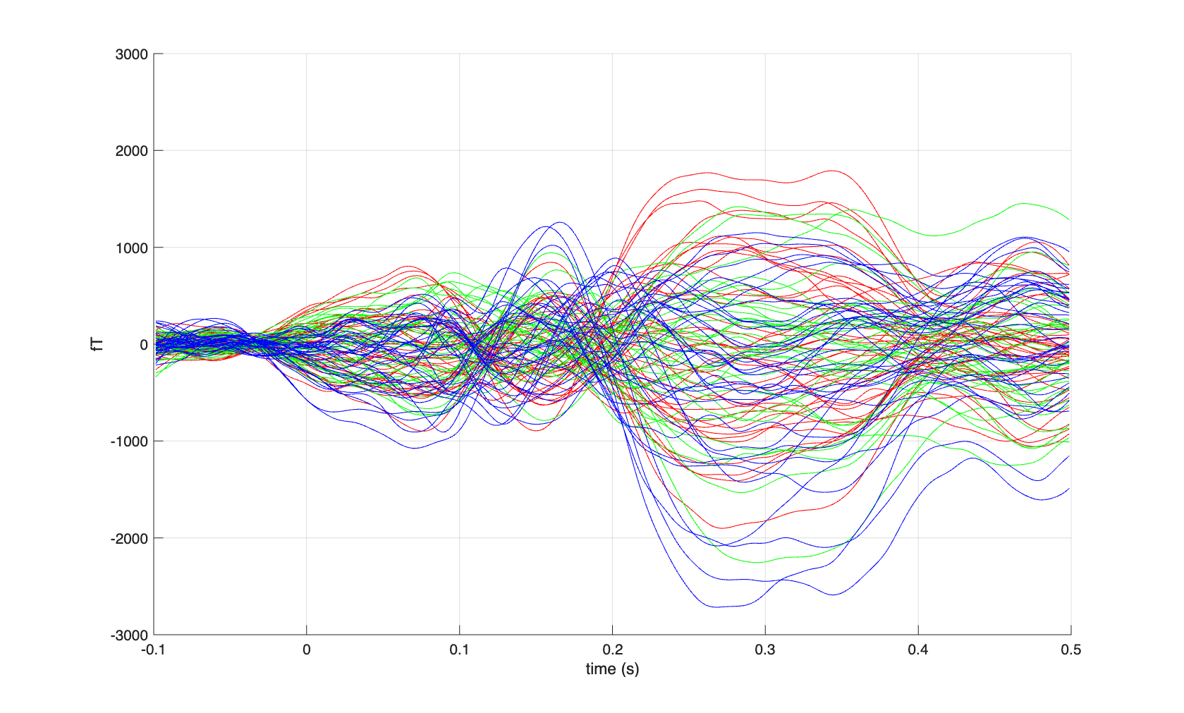
figure
hold on

sel = startsWith(timelock.label, 'X');
plot(timelock.time, timelock.avg(sel,:)*1e15, 'r');
sel = startsWith(timelock.label, 'Y');
plot(timelock.time, timelock.avg(sel,:)*1e15, 'g');
sel = startsWith(timelock.label, 'Z');
plot(timelock.time, timelock.avg(sel,:)*1e15, 'b');

grid on
ylim([-3000 3000])
xlabel('time (s)')
ylabel('fT')

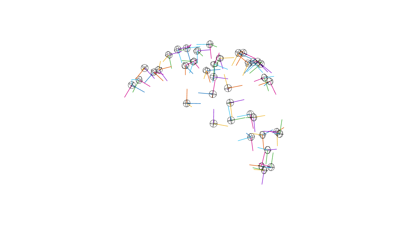
We can also plot the sensor positions, which in principle can also be used to make a topographic plot.

figure
ft_plot_sens(timelock.grad, 'orientation', true, 'coil', true)

Coregistration

QuSpin uses a semi-flexible cap or helmet that consists of multiple panels. To record the position and orientation of the sensors relative to each other, and to coregister the sensors with the head of the participant, QuSpin uses the HALO, a circular printed circuit board (PCB) containing 16 independently controllable electromagnetic coils, which is mounted above the head like an aureola.

See also

• Getting started with QuSpin OPM data