Virtual channel analysis of epilepsy MEG data

Introduction

This tutorial describes how to perform a source localization on epilepsy data using a kurtosis beamformer method implemented in FieldTrip. The tutorial assumes that the reader is already experienced with epilepsy data, and understands the basics of MEG, but is perhaps not familiar with FieldTrip or its capabilities. The tutorial does not attempt to fully explain the intrepretation of the results, which requires clinical expertise and further knowledge of the case histories.

The tutorial covers data for 3 patients, all shared via our download server. The provided datasets have varying degrees of clinical complexity. The more complex cases are, of course, the ones most likely to be referred for MEG recordings prior to consideration for surgery.

For one of the patients, case 3, we provide a detailed line-by-line breakdown of the MATLAB code required to analyze the data. We outline the steps in obtaining the beamformer outputs, from anatomical coregistration right through to plotting source images. We note an important extra step that is required in computing the beamformer for data collected on an Neuromag/Elekta/MEGIN system compared to a CTF system. We also describe how to output the source images into NiFTI format for viewing in other software such as MRIcro, and how to output source timeseries as a file which can be examined clinically alongside the original data in AnyWave data viewing software.

For patients 1 and 2, we simply provide a summary of the outputs and some other useful observations. These datasets can be analyzed by the reader in exactly the same way as case 3.

All the MEG data were recorded at Aston Brain Centre (ABC) using both a 275-channel CTF system and using a Neuromag 306-channel system. The case reports and the data are kindly provided by Professor Stefano Seri; the steps in the kurtosis pipeline itself were provided by Dr Caroline Witton on behalf of the Aston clinical team. The data have been clinically analyzed by the staff of ABC using the software accompanying the MEG systems. The FieldTrip analysis demonstrated here is only for educational purposes.

Background

The kurtosis beamformer approach described here, for identifying the source(s) of epileptiform activity, was originally published by Kirsch et al. 2006 and has subsequently been validated in other studies (e.g., Hall et al. 2017). Beamformer-based source localization can have particular advantages in cases where a wide network of cortical areas are affected, or where there is an initial lack of a priori evidence (e.g., from MRI or EEG) about the likely source of epileptogenic activity. Beamformers also provide excellent improvement in signal to noise ratio of the data.

Procedure

The Aston Brain Centre clinical staff would typically use the following sequence of analysis steps for epilepsy data:

1. Screen the data visually for spikes and also to identify physiological or external recording artifacts.
2. Choose relatively artifact-free data, that appears to contain spikes, for further analysis (bearing in mind that data quality can vary widely in patient recordings, especially children)
3. Run the kurtosis beamformer analysis to yield candidate sources in volumetric images, which can be examined alongside other information e.g., lesions visible in anatomical images.
4. Examine source time series from the candidate sources to verify the presence of spikes. Usually source time series would be visualised alongside the original raw data. Candidate spikes can be automatically marked in the time series based on their amplitude.
5. Before reporting back to the surgical team, candidate sources are typically confirmed by dipole-fitting of key spikes identified by the pipeline outlined above.

Because of the importance to clinical work of visually screening data and marking spikes, we have also incorporated here (with brief instructions) the use of AnyWave software, an open-source package for visualizing MEG and EEG data which lends itself well to the interpretation of the outputs from this analysis.

Since there are some small differences in the parameters for the beamformer analysis depending for CTF or Neuromag data, the analyzes for each data type are presented here separately.

Case 1

The data analysis for this subject shows multiple maxima in the kurtosis, and a complex pattern of epileptiform spikes. Due to the complexity of the clinical case, we will not present results here, but we will report on some details. The data is available from our download server.

Analysis of the CTF dataset

The analysis pipeline is mostly similar to that of case 3.

In the CTF recording it appears that the patient’s head is tilted to the right, relative to the coordinate axes. Apparently the anatomical landmarks at the left and right ear were not clicked symmetrically with the Polhemus. This is not a problem for further processing, as long as we remember that results are expressed in head coordinates relative to the anatomical landmark of this specific recording.

Analysis of the Neuromag dataset

In this dataset, the head coils are switched on after 20 seconds of recording, which causes a filter artifact, so we can omit the first 20 seconds of data by specifying a single ‘trial’ from 21 seconds until the end of the recording by using the ft_preprocessing function (see the line-by-line commands for case 3, below).

The joint analysis of planar and magnetometer channels for the Neuromag data did not result in satisfactory results. We chose to select only the planar gradiometers for further analysis. The results are similar, but not identical to the results from the CTF data. Both analyzes reveal an area of relatively high kurtosis adjacent to the lesion, a glioma in the right parietal area. This was the area followed up by the surgical team, based on the kurtosis data (originally analyzed in CTF software) interpreted in the context of seizure semiology and neuroanatomy. Both analyzes also yielded a strong peak in the left frontal cortex, which is also thought to be clinically significant.

In contrast with the CTF data, this analysis of the Neuromag data did not show an activation in the right frontal cortex, perhaps because of differences in the patterns of spiking activity in the different recordings, or alternatively perhaps because the patient’s head was located further from these sensors in this recording. The deeper activity that can be seen in the slice images appears to be located in white matter, but is potentially leakage from activity propagated to deeper areas e.g., insula cortex.

The flexibility of FieldTrip can offer additional information to support data interpretation. For example, the step where the MRI, sensors, head model and mesh are plotted together, can be used to examine positioning within the MEG helmet. This can be particularly important for clinical analysis with children because, with smaller heads, they can potential move quite far from the sensors. In the Maxfiltering process for the Neuromag data above, the continuous head position monitoring allowed the sensor time series to be realigned to a ‘standard’ position in the centre of the MEG helmet so this effect is not observed. However if the head position is plotted for a version of the data where this head position correction was not done, the original positioning of the brain in relation to the sensors can be seen. In this case, the patient’s head was not centrally located during the recording. This might explain the lack of activation in the right temporal lobe for this dataset and underlines the need for MEG systems which better serve pediatric recordings.

Case 2

Analysis using a pipeline similar to that for case 3 gives meaningful focal results (not presented here). The data is available from our download server.

Analysis of the CTF dataset

This follows the pipeline as described for case 3.

Analysis of the Neuromag dataset

The headshape that was scanned with the Polhemus in the Neuromag recording has a number of points where the stylus did not touch the scalp properly. These have been removed in MATLAB by hand, and the resulting headshape were written to a pos file (CTF format, ASCII) and a mat file (MATLAB).

Rather than reading the headshape from the fif file, it should be read from the mat file. Other than that the analysis follows the pipeline as described for case 3.

Case 3

The shared data is available from our download server. After downloading the data, we set up the path and ensure that FieldTrip is the only toolbox on the path. See also this FAQ.

restoredefaultpath
addpath ~/matlab/fieldtrip/
ft_defaults

datadir   = '/data/epilepsy/raw/case3'; % this contains the shared data

Analysis of the CTF dataset

We want to store all processed results in a different directory than the one containing the raw data.

outputdir = '/data/epilepsy/processed/case3'; % this is where results will be saved
cd(outputdir)

Coregistration of the MEG and MRI data

The original MRI that is provided for this patient has been partially processed with the CTF software and MRIcro, and is stored in NIFTI format. This MRI is not shared for privacy reasons. Nevertheless, here we will show how it was processed in FieldTrip.

mri_orig = ft_read_mri(fullfile(datadir, 'case3.nii'));

The dataset also includes a Polhemus recording of the head surface, which can be used to coregister the MRI to the CTF system.

filename = fullfile(datadir, 'ctf', 'case3.pos');
headshape = ft_read_headshape(filename);
headshape = ft_convert_units(headshape, 'mm');

Check the coregistration of the Polhemus headshape and the anatomical MRI. In the CTF coordinate system the x-axis should be pointing to the nose and the y-axis to the left ear.

ft_determine_coordsys(mri_orig, 'interactive', 'no')
ft_plot_headshape(headshape);

The nose in the MRI is pointing toward the +X direction, whereas the noise in the headshape is pointing in the +Y direction, i.e. the MRI is 90 degrees off with the headshape, which is in CTF coordinates.

The coregistration procedure starts with a coarse manual coregistration, followed by an automatic fine coregistration in which the skin surface from the MRI is fitted to the headshape points.

cfg = [];
cfg.method = 'headshape';
cfg.headshape.interactive = 'yes';
cfg.headshape.icp = 'yes';
cfg.headshape.headshape = headshape;
cfg.coordsys = 'ctf';
cfg.spmversion = 'spm12';
mri_realigned = ft_volumerealign(cfg, mri_orig);
mri_realigned.coordsys = 'ctf'; % remember that it is in ctf coordinates

After coregistration we check once more.

ft_determine_coordsys(mri_realigned, 'interactive', 'no')
ft_plot_headshape(headshape);

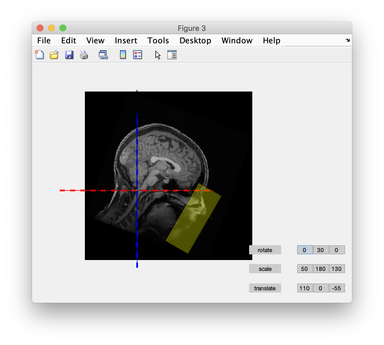
The headshape not only covers the scalp, but also the face and nose. Hence the coregistration needs to be done prior to defacing from the anatomical MRI. After coregistration we use ft_defacevolume to remove the facial details. The translate, rotate and scale parameters specified here were determined experimentally in the graphical user interface.

cfg = [];
cfg.translate = [70 0 -75];
cfg.rotate = [0 30 0];
cfg.scale = [75 175 120];
mri_defaced = ft_defacevolume(cfg, mri_realigned);

save mri_defaced.mat mri_defaced % save the data for sharing

and we use ft_volumereslice to reslice the MRI, so that the axes of the volume are aligned with the axes of the coordinate system. This facilitates plotting and ensures that results interpolated on the MRI are not displayed upside-down.

cfg = [];
mri_resliced = ft_volumereslice(cfg, mri_defaced);

save mri_resliced.mat mri_resliced % save the data for sharing

Importing and filtering the sensor level data

The kurtosis beamformer is typically run within a bandpass filter (here 10-70 Hz) which excludes some physiological artifacts such as eye blinks or EMG that might affect the analysis, while preserving as much signal from the spikes as possible. At this point we assume that the clinician has already visually screened the raw data. The current dataset is pretty clean and free of artifacts, apart from a big SQUID-jump that occurred around 50 seconds after the onset of the 2-minute recording. It is well known that the application of a filter to such a jump artifact leads to large amplitude filter ringing, with all kinds of potential consequences for the downstream analysis. Therefore, in the below, ideally we should have excluded the data segment that was affected by the SQUID-jump. However, for educational purposes, in the below we assume that the jump artifact did not affect the downstream analysis extensively, so that we don’t get stuck with the somewhat more complicated data handling that is needed to deal with this in the downstream pipeline.

dataset = fullfile(datadir, 'ctf', 'case3.ds');

cfg = [];
cfg.dataset = dataset;
cfg.hpfilter = 'yes';
cfg.hpfreq = 10;
cfg.lpfilter = 'yes';
cfg.lpfreq = 70;
cfg.channel = 'MEG';
cfg.coilaccuracy = 0; % ensure that sensors are expressed in SI units
data = ft_preprocessing(cfg);

In the following stage, we compute the data covariance matrix for the beamformer source reconstruction. We use the ft_timelockanalysis function (more commonly used elsewhere to compute an average across trials), but which can also be used to compute the covariance matrix. Unless otherwise specified in the cfg it will produce the covariance matrix for the whole time period of the data.

cfg = [];
cfg.channel = 'MEG';
cfg.covariance = 'yes';
cov_matrix = ft_timelockanalysis(cfg, data);

save cov_matrix cov_matrix

Construction of the volume conduction model of the head

We will use the defaced MRI, which has been realigned with the CTF system and resliced.

mri_resliced = ft_read_mri('mri_resliced.mat');

Segment the brain compartment from the anatomical MRI and make the volume conduction model. If you want, you can save the segmentation and head model to disk.

cfg = [];
cfg.tissue = 'brain';
cfg.spmversion = 'spm12';
seg = ft_volumesegment(cfg, mri_resliced);

save seg seg

cfg = [];
cfg.tissue = 'brain';
cfg.spmversion = 'spm12';
brain_mesh = ft_prepare_mesh(cfg, seg);

cfg = [];
cfg.method = 'singleshell';
cfg.unit = 'm'; % ensure that the headmodel is expressed in SI units
headmodel = ft_prepare_headmodel(cfg, brain_mesh);

save headmodel headmodel

Construction of the source model

To save time for the purpose of this tutorial demonstration we have chosen to use a 7 mm grid for the source model here, but in a real clinical scenario a grid of 5 mm or smaller would typically be used.

cfg = [];
cfg.headmodel = headmodel;
cfg.grad = data.grad; % this being needed here is a silly historical artifact
cfg.resolution = 0.007; % in SI units
cfg.unit = 'm'; % ensure that the sourcemodel is expressed in SI units
sourcemodel = ft_prepare_sourcemodel(cfg);

save sourcemodel sourcemodel

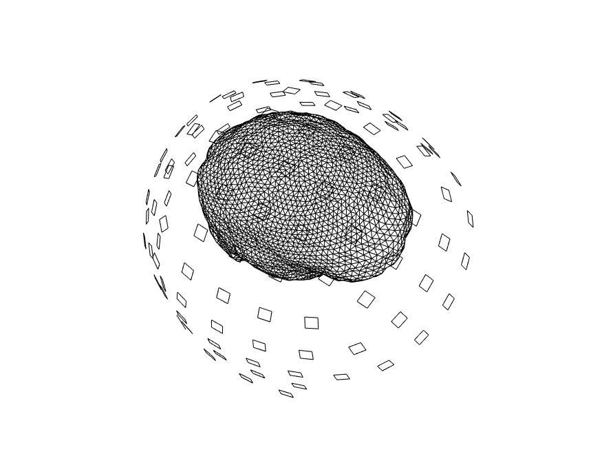
We again visualize the source model, in combination with the MRI and head model, to ensure that all geometrical data is properly aligned.

figure
ft_plot_headmodel(headmodel, 'unit', 'mm');
ft_plot_sens(data.grad, 'unit', 'mm', 'coilsize', 10, 'chantype', 'meggrad');
ft_plot_mesh(sourcemodel.pos, 'unit', 'mm');
ft_plot_ortho(mri_resliced.anatomy, 'transform', mri_resliced.transform, 'style', 'intersect', 'unit', 'mm');
alpha 0.5

Next we precompute the leadfields, which is not obligatory, but speeds up the subsequent steps.

cfg = [];
cfg.channel = 'MEG';
cfg.headmodel = headmodel;
cfg.sourcemodel = sourcemodel;
cfg.normalize = 'yes'; % normalization avoids power bias towards centre of head
cfg.reducerank = 2;
leadfield = ft_prepare_leadfield(cfg, cov_matrix);

save leadfield leadfield

Compute the beamformer virtual channels and kurtosis

Now we compute the LCMV beamformer and reconstruct the time series at each of the locations specified in the source model grid. By projecting the vector dipole moment (for x, y, and z direction) in the direction of maximal power, the source time series becomes a simple vector. The ft_sourceanalysis function can compute the kurtosis of this time series.

cfg = [];
cfg.headmodel = headmodel;
cfg.sourcemodel = leadfield;
cfg.method = 'lcmv';
cfg.lcmv.projectmom = 'yes'; % project dipole time series in direction of maximal power (see below)
cfg.lcmv.kurtosis = 'yes'; % compute kurtosis at each location
source = ft_sourceanalysis(cfg, cov_matrix);

save source source

Explore the outputs

We are ready to explore the results visually, starting with the volumetric images. First of all we need to interpolate the kurtosis on the resliced MRI, then we can plot the images. Note that the MRI is expressed in millimeter, whereas all source reconstructions are performed in SI units, i.e. in meter.

% source is in m, mri_resliced is in mm, hence source_interp will also be in mm
cfg = [];
cfg.parameter = 'kurtosis';
source_interp = ft_sourceinterpolate(cfg, source, mri_resliced);

save source_interp source_interp

cfg = [];
cfg.funparameter = 'kurtosis';
cfg.method = 'ortho'; % orthogonal slices with crosshairs at peak (default anyway if not specified)
ft_sourceplot(cfg, source_interp);

cfg = [];
cfg.funparameter = 'kurtosis';
cfg.method = 'slice'; % plot a series of slices
ft_sourceplot(cfg, source_interp);

In our figure in FieldTrip, we can scroll through the slices to see where the areas of high kurtosis fall. But to be more objective, it is useful to identify each discrete peak location in the kurtosis data. This can be done using the imregionalmax function from the Image Processing toolbox. An alternative is to use a 3rd party function called findpeaksn.m which needs to be downloaded separately and added to the MATLAB path. The Aston clinical team would typically examine every single peak but for simplicity we will just look at the top few. We display the co-ordinates and plot some images.

We use a bit of standard MATLAB code to find the regional peaks in the kurtosis

array = reshape(source.avg.kurtosis, source.dim);
array(isnan(array)) = 0;
ispeak = imregionalmax(array); % findpeaksn is an alternative that does not require the image toolbox
peakindex = find(ispeak(:));
[peakval, i] = sort(source.avg.kurtosis(peakindex), 'descend'); % sort on the basis of kurtosis value
peakindex = peakindex(i);

npeaks = 10;
disp(source.pos(peakindex(1:npeaks),:)); % output the positions of the top peaks

for i = 1:npeaks
  cfg = [];
  cfg.funparameter = 'kurtosis';
  cfg.location = source.pos(peakindex(i),:)*1000; % convert from m into mm
  ft_sourceplot(cfg, source_interp);
end

Visualize the kurtosis images in MRIcro

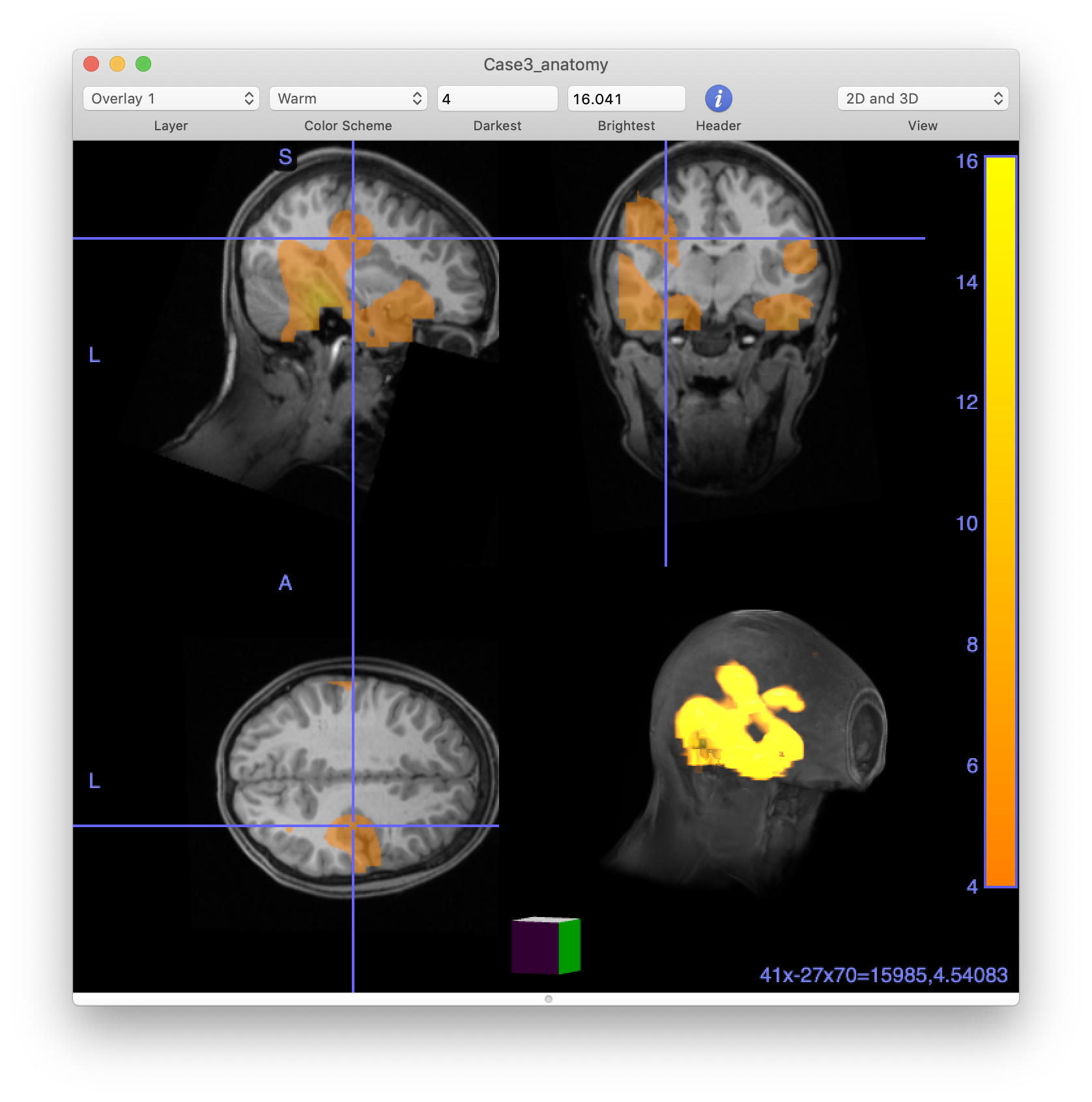
At this stage, we can also write out our images (i.e., the resliced MRI and the kurtosis image that we just made) into NIFTI format so they can be imported into other software that may be more prevalent in clinical settings and allows the results to merged with other clinical information.

cfg = [];
cfg.filename = 'Case3_anatomy.nii';
cfg.parameter = 'anatomy';
cfg.format = 'nifti';
ft_volumewrite(cfg, source_interp);

cfg = [];
cfg.filename = 'Case3_kurtosis.nii';
cfg.parameter = 'kurtosis';
cfg.format = 'nifti';
cfg.datatype = 'float'; % integer datatypes will be scaled to the maximum, floating point datatypes not
ft_volumewrite(cfg, source_interp);

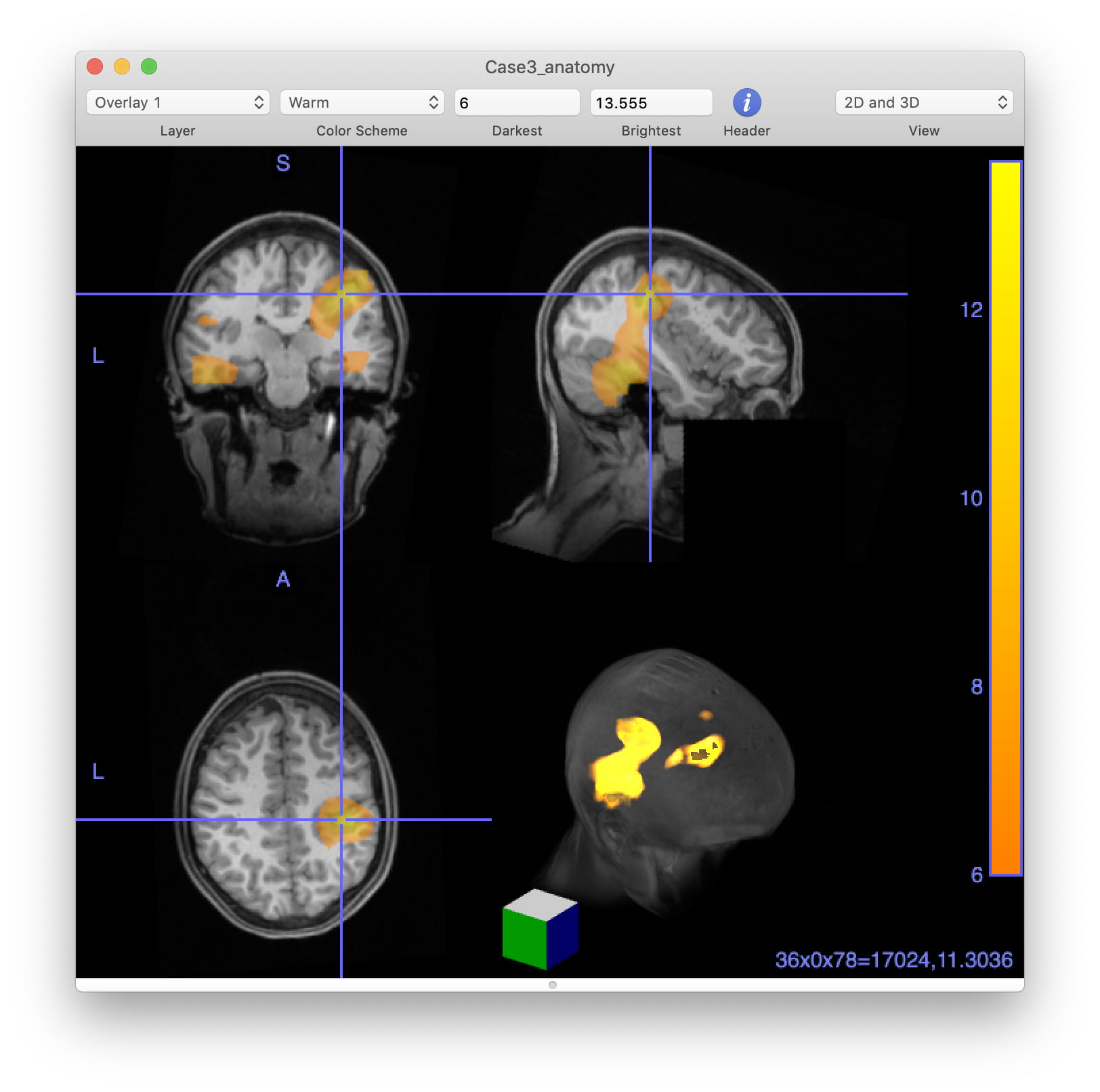
The MRIcro software from Chris Rorden’s lab is very useful to visualize anatomical in combination with functional data, to change thresholds on the fly, and to make 3D renderings of the peaks of the activity in relation to the anatomy.

Visualize the beamformer time series in AnyWave

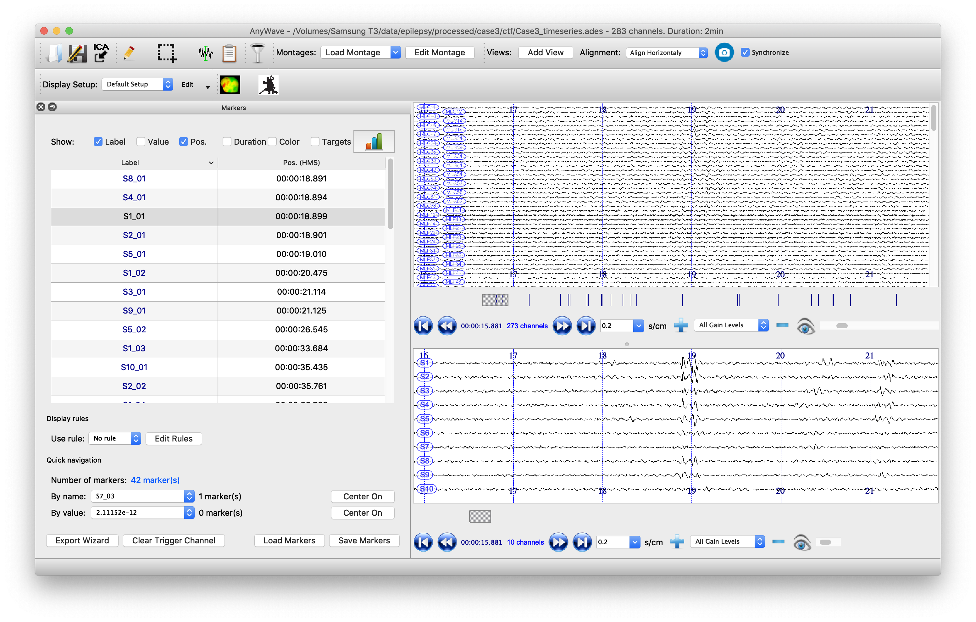
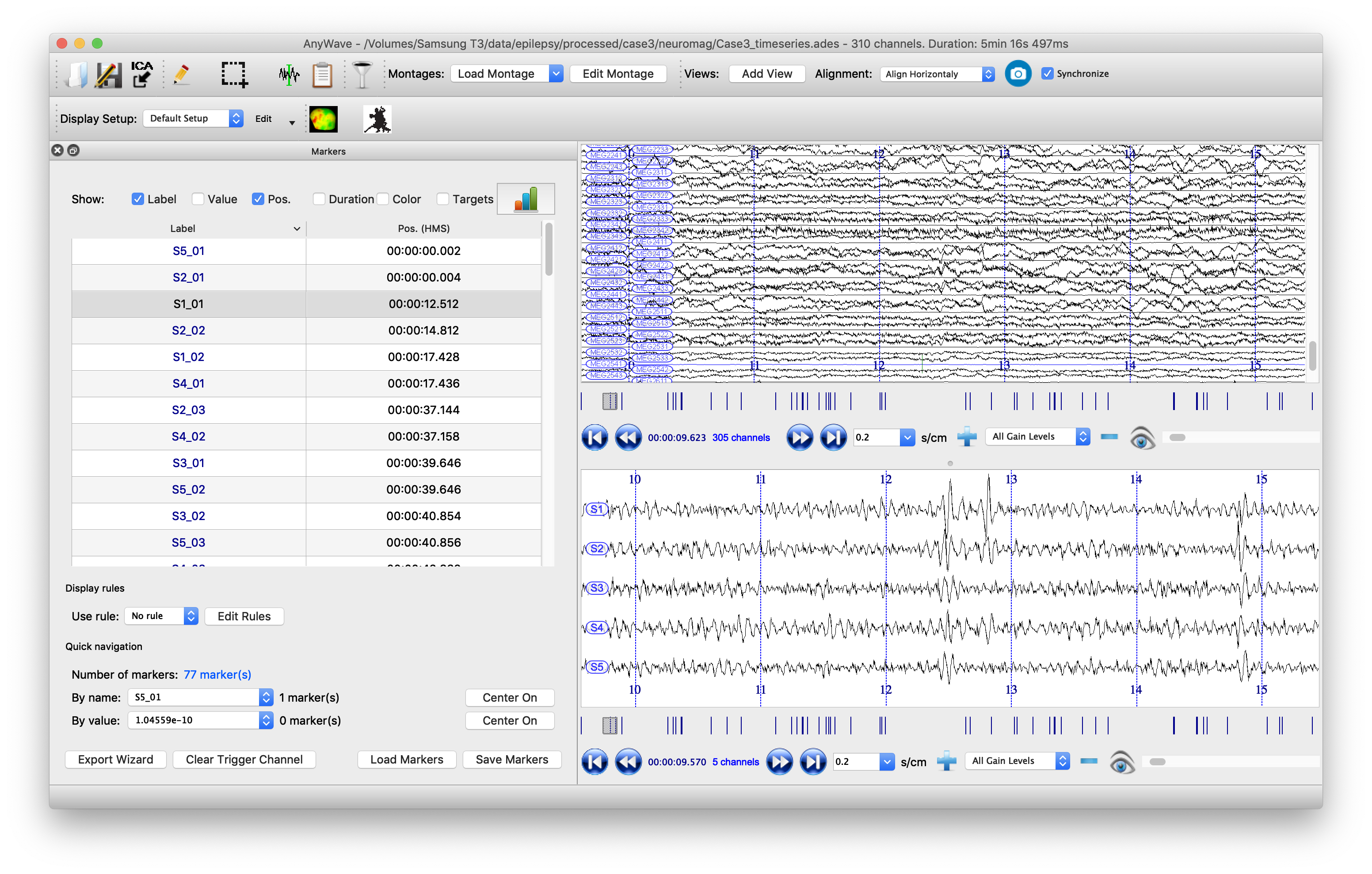
It is also clinically important to visualize the spikes that are contributing to the kurtosis images, not least to screen out any spurious sources which may be elicited by artifacts. To do this, it is useful to have the original sensor data visible alongside the source time series. Marking the timepoints at which spikes occur at the sources can help the clinician scroll more easily through the data. We will write the data to a format that can be read by the open-source package AnyWave, which is well-suited to this purpose.

When we read in the data earlier, we filtered it, but here it is more useful to have the unfiltered data. So we import that to FieldTrip and then append source time series data, adding header information for this, before writing the whole lot to the AnyWave ADES file format.

cfg = [];
cfg.dataset = dataset;
cfg.channel = 'MEG';
cfg.coilaccuracy = 0;
data_unfiltered = ft_preprocessing(cfg);

dat = ft_fetch_data(data_unfiltered);
hdr = ft_fetch_header(data_unfiltered);

npeaks = 10; % for simplicity we limit ourselves to appending the time series of the top peaks
for i = 1:npeaks
  dat(end+1,:)= source.avg.mom{peakindex(i),:}; % see note below about scaling
  hdr.label{end+1}= ['S' num2str(i)];
  hdr.chantype{end+1} = 'Source';
  hdr.chanunit{end+1} = 'T'; % see note below about scaling
end
hdr.nChans = hdr.nChans+npeaks;
ft_write_data('Case3_timeseries', dat, 'header', hdr, 'dataformat', 'anywave_ades');

Finally we can automatically mark potential spikes in the source time series data and create labels in AnyWave marker file format. We use the convention (from the original CTF SAMg2 software) of placing a marker wherever the source time series exceeds 6 standard deviations of its mean. In our marker file, there is one label for each source, so events on the marker labeled ‘S1’ correspond to spikes on the time series from peak number 1 in the image. Marker S2 indicates events occurring at peak number 2, etc., etc.

fid = fopen('Case3_timeseries.mrk', 'w');
fprintf(fid,'%s\r\n','// AnyWave Marker File ');
k = 1;
for i = 1:npeaks
  dat = source.avg.mom{peakindex(i),:};
  sd = std(dat);
  tr = zeros(size(dat));
  tr(dat>6*sd)=1;
  [tmp, peaksample] = findpeaks(tr, 'MinPeakDistance', 300); % peaks have to be separated by 300 sample points to be treated as separate
  for j = 1:length(peaksample)
    fprintf(fid, 'S%d_%02d\t', i, j); % marker name
    fprintf(fid, '%d\t', dat(peaksample(j))); % marker value
    fprintf(fid, '%d\t',source.time(peaksample(j)) ); % marker time
    fprintf(fid, '%d\t', 0); % marker duration
    fprintf(fid, 'S%d\r\n', i); % marker channel
    k = k + 1;
  end
end
fclose(fid);

The data can now be opened in AnyWave. Once the file is opened, to see sources alongside source data, click ‘Add View’ in the top/middle toolbar. Then use the eyeball icon to set each view so that one has ‘MEG’ and one has ‘SOURCE’ data. Set the timescale to be 0.3 sec/cm (close to the clinical standard 3cm/sec) and scale the amplitudes appropriately. Use the menu to import the marker file that we just created.

Analysis of the Neuromag dataset

The Neuromag (formerly also known as ‘Elekta’ and now operating under the company name ‘MEGIN’) dataset was collected from the same patient on the same day as the CTF dataset described above. So, we expect the results to be very similar to those yielded by the CTF data.

Generally the analysis of Neuromag data is almost identical to the analysis of CTF data. So this part of the tutorial has fewer comments than above. However there is one important difference, related to the processing of Maxfiltered data, which is addressed in more detail in the relevant tutorial sections below. Maxfilter is proprietary software that comes with the Neuromag system for pre-processing; it offers some improvements in signal-to-noise ratio and artifact handling, and potential for head movement correction. Importantly it is obligatory in datasets where active shielding (‘MaxShield’) was used during data collection and indeed the epilepsy data used here required preprocessing with Maxfilter for this reason. But Maxfilter has effects on the data covariance which can cause problems in accurately computing the beamformer source model. Some ways to optimize the beamformer calculations to avoid these problems are demonstrated below.

To ensure that we are not mixing up the two datasets, we will clear all variables from MATLAB memory and start from scratch.

clear all

datadir   = '/data/epilepsy/raw/case3'; % this contains the shared data

outputdir = '/data/epilepsy/processed/case3/neuromag';
cd(outputdir)

Coregistration of the MRI data to the MEG data

For patient confidentiality we only include here the MRI which has already been coregistered with the data, defaced, and resliced to align it to the data head co-ordinate system. The process for coregistration is identical to the one described above, except that in the Neuromag system the Polhemus head shape points are stored in the raw data file.

mri_orig = ft_read_mri(fullfile(datadir, 'case3.nii'));

headshape = ft_read_headshape(fullfile(datadir, 'neuromag', 'case3.fif'));
headshape = ft_convert_units(headshape, 'mm');

ft_determine_coordsys(mri_orig, 'interactive', 'no')
ft_plot_headshape(headshape);

cfg = [];
cfg.method = 'headshape';
cfg.headshape.interactive = 'yes';
cfg.headshape.icp = 'yes';
cfg.headshape.headshape = headshape;
cfg.coordsys = 'neuromag';
cfg.spmversion = 'spm12';
mri_realigned = ft_volumerealign(cfg, mri_orig);
mri_realigned.coordsys = 'neuromag'; % remember that it is in neuromag coordinates

% Do you want to change the anatomical labels for the axes [Y, n]? y
% What is the anatomical label for the positive X-axis [r, l, a, p, s, i]? r
% What is the anatomical label for the positive Y-axis [r, l, a, p, s, i]? a
% What is the anatomical label for the positive Z-axis [r, l, a, p, s, i]? s
% Is the origin of the coordinate system at the a(nterior commissure), i(nterauricular), n(ot a landmark)? i

ft_determine_coordsys(mri_realigned, 'interactive', 'no')
ft_plot_headshape(headshape);

cfg = [];
cfg.translate = [0 70 -60];
cfg.rotate = [0 0 0];
cfg.scale = [150 100 120];
mri_defaced = ft_defacevolume(cfg, mri_realigned);

save mri_defaced.mat mri_defaced % save the data for sharing

When we reslice this MRI, it becomes aligned with the Neuromag co-ordinate system (RAS) which means that slice images are shown in a different set of orientations to the CTF data that has been aligned to its own co-ordinate system. See this FAQ for more details on different coordinate systems.

cfg = [];
mri_resliced = ft_volumereslice(cfg, mri_defaced);

save mri_resliced.mat mri_resliced % save the data for sharing

Importing and filtering the sensor level data

Neuromag MEG data has two channel types - magnetometers and planar gradiometers - and in this analysis we use both at the same time. The units of planar magnetometers (field per distance) are different than the units of magnetometers (field), therefore we have to use SI units to ensure that all forward and inverse model computations are correct.

We apply the same 10-70 Hz bandpass filter as for the CTF analysis.

dataset = fullfile(datadir, 'neuromag', 'case3.fif');

cfg = [];
cfg.dataset = dataset;
cfg.hpfilter = 'yes';
cfg.hpfreq = 10;
cfg.lpfilter = 'yes';
cfg.lpfreq = 70;
cfg.channel = {'megmag', 'meggrad'};
cfg.coilaccuracy = 0;
data = ft_preprocessing(cfg);

The data comprises 300 seconds at 2000Hz, which results in a 16GB source reconstruction in memory. Although this is is fine for clinical work on heavy workstations, for demonstration purposes we will downsample the data here to reduce the memory requirements.

cfg = [];
cfg.resamplefs = 500;
data_resampled = ft_resampledata(cfg, data);

We compute the data covariance window as before.

cfg = [];
cfg.channel = 'MEG';
cfg.covariance = 'yes';
cov_matrix = ft_timelockanalysis(cfg, data_resampled);

save cov_matrix cov_matrix

Construction of the volume conduction model of the head

This follows the same procedure as for the CTF data

mri_resliced = ft_read_mri('mri_resliced.mat');

cfg = [];
cfg.tissue = 'brain';
cfg.spmversion = 'spm12';
seg = ft_volumesegment(cfg, mri_resliced);

save seg seg

cfg = [];
cfg.tissue = 'brain';
cfg.spmversion = 'spm12';
brain_mesh = ft_prepare_mesh(cfg, seg);

cfg = [];
cfg.method = 'singleshell';
headmodel = ft_prepare_headmodel(cfg, brain_mesh);

save headmodel headmodel

Construction of the source model

cfg = [];
cfg.resolution = 0.007; % clinical work would typically use a grid which <5mm
cfg.unit = 'm';
cfg.headmodel = headmodel;
cfg.grad = data.grad;
sourcemodel = ft_prepare_sourcemodel(cfg);

save sourcemodel sourcemodel

cfg = [];
cfg.channel = 'MEG';
cfg.headmodel = headmodel;
cfg.sourcemodel = sourcemodel;
cfg.normalize = 'yes'; % normalisation avoids power bias towards centre of head
cfg.reducerank = 2;
leadfield = ft_prepare_leadfield(cfg, cov_matrix);

save leadfield leadfield

Again we plot all geometrical data to check their alignment.

figure
ft_plot_axes([], 'unit', 'mm', 'coordsys', 'neuromag');
ft_plot_headmodel(headmodel, 'unit', 'mm'); % this is the brain shaped head model volume
ft_plot_sens(data.grad, 'unit', 'mm', 'coilsize', 10); % the sensor locations
ft_plot_mesh(sourcemodel.pos, 'unit', 'mm'); % the source model is a cubic grid of points
ft_plot_ortho(mri_resliced.anatomy, 'transform', mri_resliced.transform, 'style', 'intersect');
alpha 0.5 % make the anatomical MRI slices a bit transparent

Compute the beamformer virtual channels and kurtosis

At this point the analysis deviates from the CTF analysis because we need to account for differences in the covariance matrix that result from Maxfilter. First, we perform a singular value decomposition of the covariance matrix and plot the singular values, ‘s’. These are plotted in descending order, and the discontinuity that occurs after the 68th value reflects the effects of Maxfilter, which has reconstructed the data based on (typically) about 80 components.

[u,s,v] = svd(cov_matrix.cov);
figure;
semilogy(diag(s),'o-');

As we compute the LCMV beamformer below, we can use the information from the SVD to help regularize the covariance matrix using a truncation parameter called kappa. We set this at a value before the big ‘cliff’ in the singular values. We also set a parameter called lambda which can be considered a weighting factor for the regularization.

cfg = [];
cfg.method = 'lcmv';
cfg.sourcemodel = leadfield;
cfg.headmodel = headmodel;
cfg.lcmv.keepfilter = 'yes';
cfg.lcmv.fixedori = 'yes'; % project on axis of most variance using SVD
cfg.lcmv.lambda = '5%';
cfg.lcmv.kappa = 69;
cfg.lcmv.projectmom = 'yes'; % project dipole time series in direction of maximal power (see below)
cfg.lcmv.kurtosis = 'yes';
source = ft_sourceanalysis(cfg, cov_matrix);

save source source

Explore the results

The remainder of the analysis is identical to the CTF analysis: we interpolate and export the images and the time series.

cfg = [];
cfg.parameter = 'kurtosis';
source_interp = ft_sourceinterpolate(cfg, source, mri_resliced);

cfg = [];
cfg.funparameter = 'kurtosis';
cfg.method = 'ortho'; % orthogonal slices with crosshairs at peak (default anyway if not specified)
ft_sourceplot(cfg, source_interp);

cfg = [];
cfg.funparameter = 'kurtosis';
cfg.method = 'slice'; % plot slices
ft_sourceplot(cfg, source_interp);

array = reshape(source.avg.kurtosis, source.dim);
array(isnan(array)) = 0;
ispeak = imregionalmax(array); % findpeaksn is an alternative that does not require the image toolbox
peakindex = find(ispeak(:));
[peakval, i] = sort(source.avg.kurtosis(peakindex), 'descend'); % sort on the basis of kurtosis value
peakindex = peakindex(i);

npeaks = 5;
disp(source.pos(peakindex(1:npeaks),:)); % output their positions

for i = 1:npeaks
  cfg = [];
  cfg.funparameter = 'kurtosis';
  cfg.location = source.pos(peakindex(i),:)*1000; % convert from m to mm
  ft_sourceplot(cfg, source_interp);
end

Visualize the kurtosis images in MRIcro

cfg = [];
cfg.filename = 'Case3_anatomy.nii';
cfg.parameter = 'anatomy';
cfg.format = 'nifti';
ft_volumewrite(cfg, source_interp);

cfg = [];
cfg.filename = 'Case3_kurtosis.nii';
cfg.parameter = 'kurtosis';
cfg.format = 'nifti';
cfg.datatype = 'float'; % integer datatypes will be scaled to the maximum, floating point datatypes not
ft_volumewrite(cfg, source_interp);

Visualize the beamformer time series in AnyWave

cfg = [];
cfg.dataset = dataset;
cfg.channel = 'MEG';
cfg.coilaccuracy = 0;
data_unfiltered = ft_preprocessing(cfg);

cfg = [];
cfg.resamplefs = 500;
data_unfiltered_resampled = ft_resampledata(cfg, data_unfiltered);

dat = ft_fetch_data(data_unfiltered_resampled);
hdr = ft_fetch_header(data_unfiltered_resampled);

npeaks = 5;
for i = 1:npeaks
  dat(end+1,:) = source.avg.mom{peakindex(i),:}; % see comment below about scaling
  hdr.label{end+1}= ['S' num2str(i)];
  hdr.chantype{end+1} = 'Source';
  hdr.chanunit{end+1} = 'T' ; % see note below about scaling
end
hdr.nChans = hdr.nChans+npeaks;
ft_write_data('Case3_timeseries', dat, 'header', hdr, 'dataformat', 'anywave_ades');

fid = fopen('Case3_timeseries.mrk', 'w');
fprintf(fid,'%s\r\n','// AnyWave Marker File ');
k = 1;
for i = 1:npeaks
  dat = source.avg.mom{peakindex(i),:};
  sd = std(dat);
  tr = zeros(size(dat));
  tr(dat>6*sd)=1;
  [tmp, peaksample] = findpeaks(tr, 'MinPeakDistance', 300); % peaks have to be separated by 300 sample points to be treated as separate
  for j = 1:length(peaksample)
    fprintf(fid, 'S%d_%02d\t', i, j); % marker name
    fprintf(fid, '%d\t', dat(peaksample(j))); % marker value
    fprintf(fid, '%d\t',source.time(peaksample(j)) ); % marker time
    fprintf(fid, '%d\t', 0); % marker duration
    fprintf(fid, 'S%d\r\n', i); % marker channel
    k = k + 1;
  end
end
fclose(fid);

Summary and Conclusions

This tutorial provided step-by-step details on how to perform a kurtosis beamformer analysis of epilepsy data using FieldTrip. Data for 3 patients were shared, and detailed analysis instructions were given for Patient 3. As well as outlining how the data are processed in FieldTrip, the tutorial described how to write the outputs into file formats which can be read with other software, to continue the clinical interpretation of the data.

As a next step, the reader can use the steps given for Patient 3 to analyze the data for the other two patients, as a proof-of-concept.

In conclusion, this tutorial illustrates how the capabilities of FieldTrip are well suited to the requirements of epilepsy data analysis, and provide a clear and transparent pipeline that is easily applied.