Analysis of monkey ECoG recordings
Introduction
In the following tutorial we will analyze a whole hemisphere EcoG grid implanted in a macaque monkey. This data set has been recorded in the Laboratory for Adaptive Intelligence, BSI, RIKEN, Japan and has been shared as part of the NeuroTycho project. The NeuroTycho homepage also provides some information about why and how the data is shared so that we will not expand on this here. Instead this tutorial provides some overview of how to get started with ECoG data by using this particular data set as an example.
Background
This particular experiment deals with a visual grating task. This particular task is known to reliably elicit a sustained signal in the gamma frequency range ~60-80 Hz in both humans and nonhuman primates. More elaborate discussion on the sustained gamma band signal can be found here. The animal is seated with fixated head and restrained arm motion in front of a black screen. A grating pattern in eight different orientation has been presented for 2 seconds following a 2 seconds baseline period (black screen) while the brain activity was monitored with 128 channel ECoG grid covering the entire right hemisphere (Figure1). Some more information can be found here, where you can also download the data.
Figure 1: X-ray with electrode coverage illustrating the position of the electrodes in the right hemisphere
Procedure
The tutorial will follow the steps:
- prepare a 2D electrode layout for visualization that will be used throughout the tutorial with ft_prepare_layout and plot it with ft_layoutplot
- load data into MATLAB and assemble it into a format FieldTrip can deal with
- define a trial structure and subsequently use ft_redefinetrial in order to separate the eight conditions/orientations.
- append the data into a common dataset ft_appenddata apply an independent component analysis using ft_componentanalysis after which we will plot and explore some components using ft_databrowser
- Compute time-frequency representations of power and plot using ft_freqanalysis and ft_multiplotTFR respectively.
- Compute coherence between reference electrode and the remaining electrodes using ft_connectivityanalysis.
- Perform networkanalysis using ft_networkanalysis
Preprocessing
First we will generate the layout along the guidelines explained in the layout tutorial here. Once you have downloaded and uncompressed the data you can load and restructure it in the following way. Alternatively you can download the reformatted data here.
load Event.mat
load lay
vec=1:128;
for i=1:length(vec)
 filename=strcat('ECoG_ch', num2str(vec(i)));
 data.label{i} = num2str(vec(i));
 load(filename)
 filename2 = strcat('ECoGData_ch', num2str(vec(i)));
 data.trial(i,:) = eval(filename2);
 data.time = {EventTime};
 data.fsample = 1000;
end

data.trial = {data.trial};
data.label = lay.label(1:128);
data.trial = double(data.trial{1})
data.trial = {data.trial};
data.label{129} = 'event';
clear ECoG*
Using the information provided in the “readme.txt” file, we can build a trial structure that can be used during the call to ft_redefinetrial
trigger = EventData;
sample  = EventIndex;

% determine the number of samples before and after the trigger
pretrig  = -data.fsample*2;
posttrig =  data.fsample*2;

trl = [];
for j = 2:(length(trigger)-2)
  trg1 = trigger(j);
  trg2 = trigger(j+1);
  trg3 = trigger(j+1);
  trg4 = trigger(j-1);

  %%% provided txt file reads that
  %%% orientation one spans values from 650 to 750
  %%% baseline spans values from 300 400

  if trg1 > 400 && trg2 `< 750 && trg3 >`= 650 && trg4 <= 400
    trlbegin = sample(j) + pretrig;
    trlend   = sample(j) + posttrig;
    offset   = pretrig;
    newtrl   = [trlbegin trlend offset];
    trl      = [trl; newtrl];
  end
end
The structure trl is now a 20 rows by 3 columns matrix containing the begin, end and offset(i.e. baseline) samples for each trial of type 45° orientation. Subsequently we call ft_redefinetrial where we provide the trial structure computed in the previous step cfg.trl = trl;.
cfg     = [];
cfg.trl = trl;
data_1 = ft_redefinetrial(cfg,data);
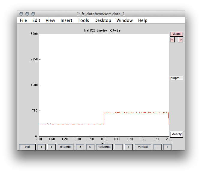
Now we illustrate the time course of the channel defining the event in order to check whether trial onset was appropriately assigned.
cfg           = [];
cfg.trl       = data_1.trial;
cfg.channel   = 'event';
cfg.ylim      = [0 3000];
cfg.blocksize = 4;
ft_databrowser(cfg, data_1);
Figure 2: Event onset at time stamp 0 and duration 2 seconds.
Next, we will use independent component analysis to identify the presence of artifacts but also the presence of oscillatory activity. First, the data is resampled down to 140 Hz in order to speed up the calculation of the independent components. We reduce the iteration steps to 50 and finally project the original high sampling data thru the identified components again.
%% resample the data
cfg            = [];
cfg.resamplefs = 140;
cfg.detrend    = 'no';
datads = ft_resampledata(cfg, data);

% decompose the data
cfg                 = [];
cfg.method          = 'runica';
cfg.runica.maxsteps = 50;
comp = ft_componentanalysis(cfg, datads);

% project the original data thru the components again
cfg           = [];
cfg.unmixing  = comp.unmixing;
cfg.topolabel = comp.topolabel;
comp = ft_componentanalysis(cfg, data);
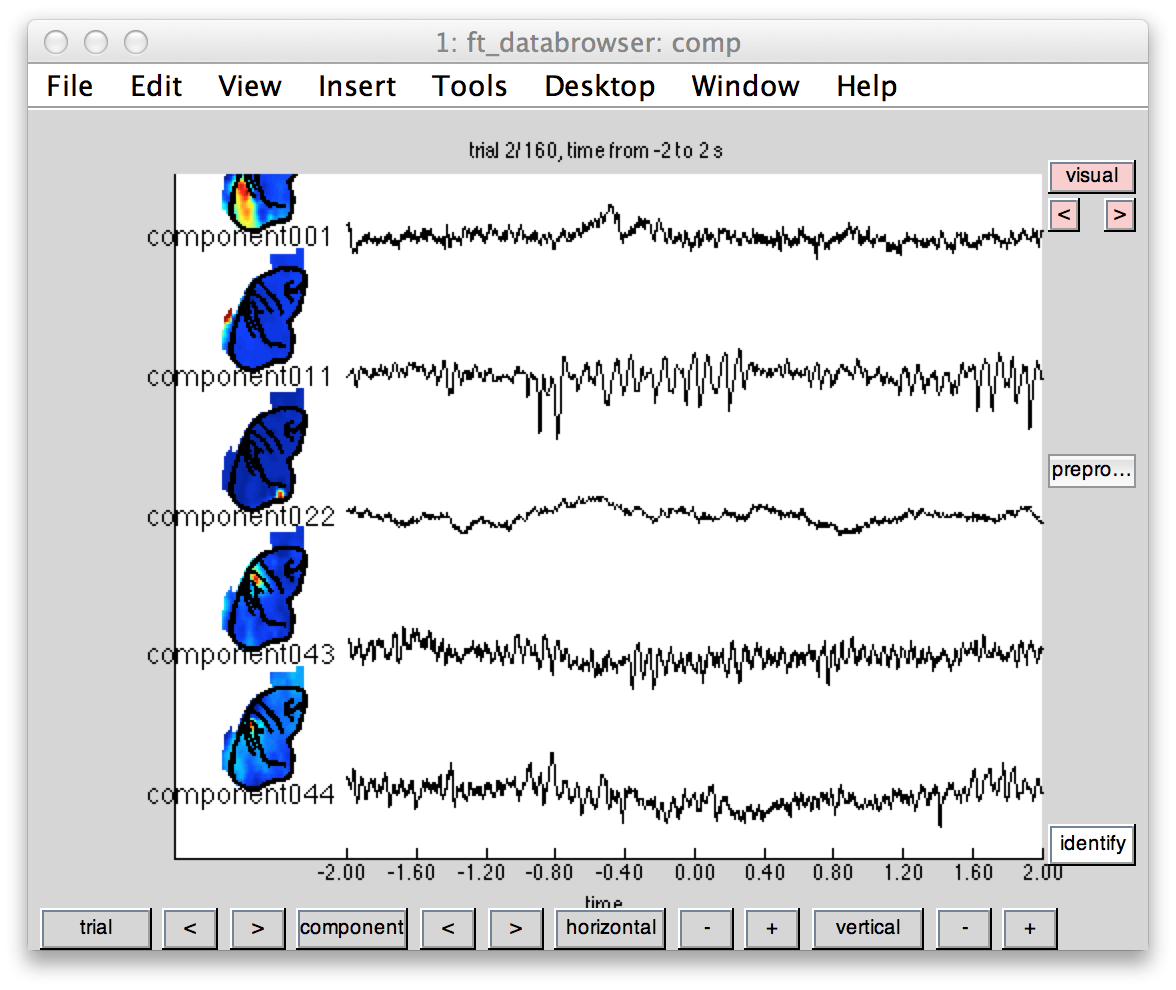
We will use ft_databrowser again in order to plot the topography of the components and corresponding time courses. In the present case only particular components bearing artifacts (component 22) and clear oscillatory signatures (11,43,44) are plotted.
Figure 3: Independent components illustrating some clear visual (1 and 11) and sensorimotor (43,44) topography and oscillatory time course.
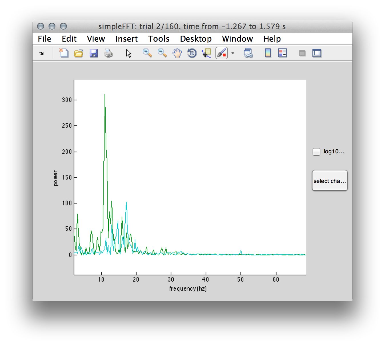
The build-in functionality of ft_databrowser allows for interactively mark a time window and perform a spectral analysis via left mouse click. This launches an additional figure that allows for adding and removing of component’s power spectra and (log/linear) scale adjustments. Doing so we can confirm the presence of 10.89 Hz alpha peak (compontent 11) over occipito-posterior electrodes (component 11 topography in Figure 3).
Figure 4: Power spectrum of components #11 and #43 illustrating a clear 10.89 Hz alpha peak (green traces) in the visual and 17.05 beta peak (cyan traces) in the sensorimotor regions.
Time-frequency analysis
After rejecting bad components with ft_rejectcomponent a time-frequency analysis can be performed. Detailed information regarding this analysis step is extensively covered here. Furthermore, we will use different settings for the estimates of low (<40Hz) and high (>40Hz) frequencies. The rational behind this strategy is also covered in the time-frequency tutorial and extensively explained by Robert in the video lecture here. The time-frequency representation of power is calculated with ft_freqanalysis. Subsequently the power estimates are baseline corrected with ft_freqbaseline and plotted with ft_multiplotTFR.
% perform time-frequency analysis
cfg              = [];
cfg.output       = 'pow';
cfg.method       = 'mtmconvol';
cfg.taper        = 'hanning';
cfg.foi          = 1:1:40;
cfg.t_ftimwin    = ones(length(cfg.foi),1).*0.5;
cfg.toi          = -2:0.05:2;
cfg.keeptrials   ='yes';
tfr = ft_freqanalysis(cfg,data);

% baseline correction
cfg               = [];
cfg.baseline      = [-1 0];
cfg.baselinetype  = 'db';
tfrbl = ft_freqbaseline(cfg, tfr);

% plot the result
cfg           = [];
cfg.channel   = {'all'};
cfg.xlim      = [-.2 2];
cfg.ylim      = [1 40];
cfg.fontsize  = 12;
cfg.layout    = lay;
% cfg.zlim    = [-.5 .5];
figure;
ft_multiplotTFR(cfg, tfrbl);
Figure 5: Time-frequency representation of power using ft_multiplotTFR and the layout designed in the steps above. Highlighted area of electrodes is used for the illustration in figure 6.
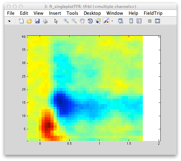
Figure 6: Time-frequency representation of power averaged across the electrodes highlighted in the previous figure. Note the initial evoked power in the low frequency range followed by induced depression of oscillatory power in the alpha frequency range.
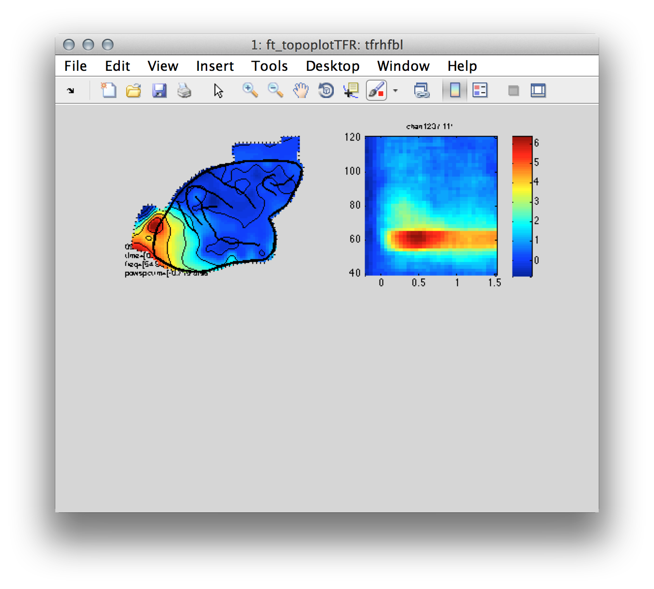
Typically, visual grating tasks reliably elicit sustained gamma band response ~60-80 Hz in both humans (Hoogenboom N1, Schoffelen JM, Oostenveld R, Parkes LM, Fries P. (2006) Localizing human visual gamma-band activity in frequency, time and space. Neuroimage. 2006 Feb 1;29(3):764-73. Epub 2005 Oct 10.) and non human primates (Fries P, Scheeringa R, Oostenveld R. (2008) Finding Gamma. Neuron. 2008 May 8;58(3):303-5. doi: 10.1016/j.neuron.2008.04.020.). The following lines will estimate oscillatory power in the higher frequencies > 40 Hz, baseline correct and plot the rusult.
% estimate high frequency gamma
cfg            = [];
cfg.output     = 'pow';
cfg.method     = 'mtmconvol';
cfg.taper      = 'dpss';
cfg.foi        = 40:2:120;
cfg.t_ftimwin  = ones(length(cfg.foi),1).*0.5;
cfg.tapsmofrq  = 6 ;
cfg.toi        = -2:0.05:2;
cfg.pad        = 'maxperlen';
cfg.keeptrials = 'yes';
tfrhf = ft_freqanalysis(cfg, data);

% baseline correct
cfg              = [];
cfg.baseline     = [-.75 0];
cfg.baselinetype = 'db';
tfrhfbl = ft_freqbaseline(cfg, tfrhf);

% plot
figure;
cfg         = [];
cfg.xlim    = [0.18 0.87]
cfg.ylim    = [53 80];
cfg.layout  = lay;
subplot(2,2,1); ft_topoplotTFR(cfg,tfrhfbl);
cfg         = [];
cfg.channel = {'chan123'};
cfg.xlim    = [-.2 1.5];
cfg.ylim    = [40 120];
subplot(2,2,2); ft_singleplotTFR(cfg,tfrhfbl);
Figure 7: Left- topography of the induced gamma band response centered around ~60 Hz. Right-Time-frequency representation of power for a single electrode located over the occipital cortex.
Connectivity analysis
Now we can analysis the connectivity patterns that may arise due to coherence in the gamma band. Towards this end we’ll use ft_connectivityanalysis and imaginary coherence as a metric of communication between electrodes. First, we take advantage of multitapering in order to estimated gamma power at 60 Hz and compute the connectivity between all possible electrode pairs.
% estimate 60 Hz power
cfg            = [];
cfg.method     = 'mtmfft';
cfg.output     = 'fourier';
cfg.taper      = 'dpss';
cfg.keeptrials = 'yes';
cfg.tapsmofrq  = 2;
cfg.foi        = 60;
freq           = ft_freqanalysis(cfg, data);

% then compute connectivity
cfg         = [];
cfg.method  = 'coh';
cfg.complex = 'absimag'; % check absimag solves the abs on line 161
conn = ft_connectivityanalysis(cfg,freq);
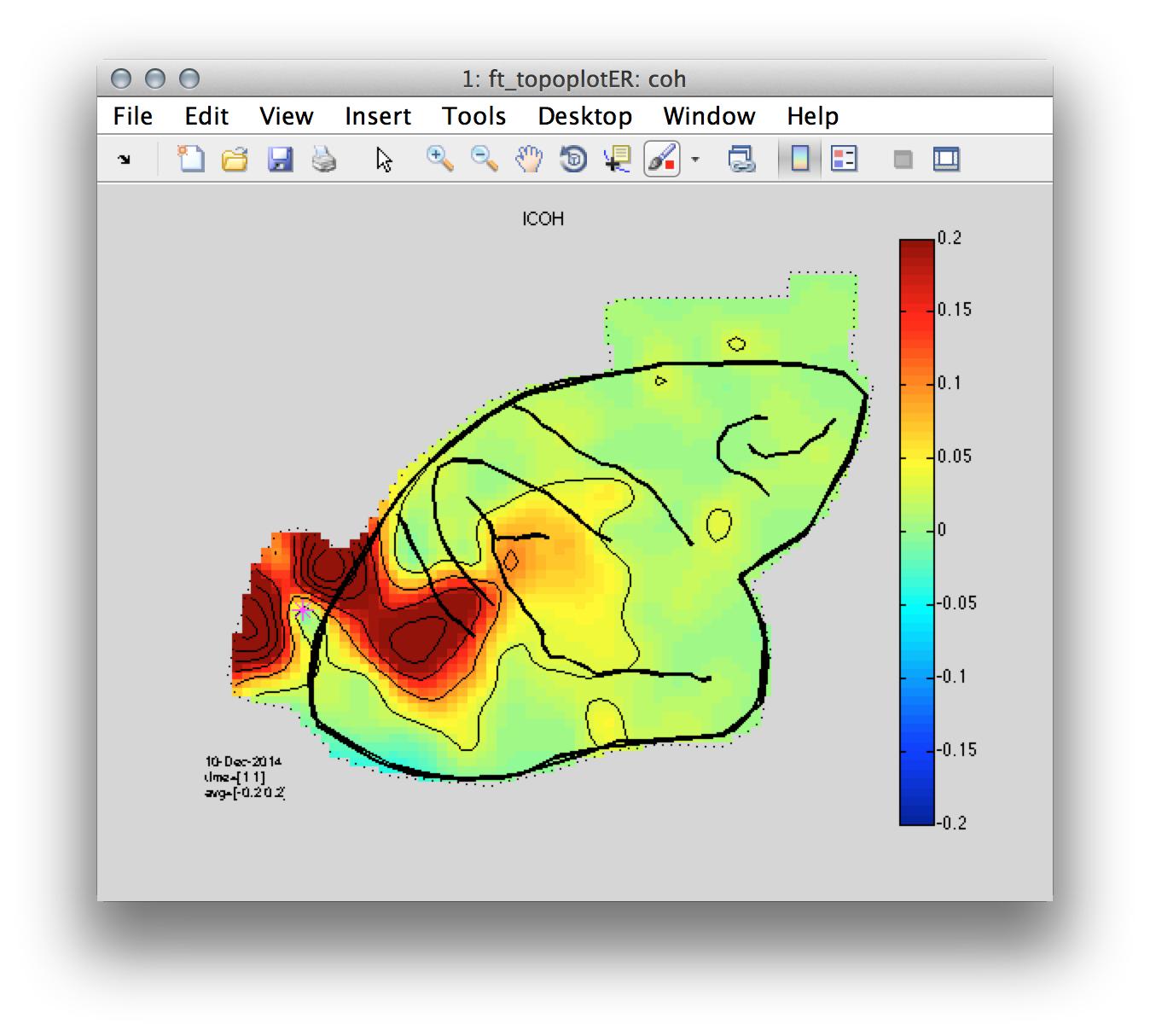
Now we plot the coherence of a reference electrode with maximal gamma power relative to the remaining electrodes. In this case the electrode is ‘chan123’ with an index number 119.
%% plot coherence from max gamma chan to all other
coh.label =data.label;
coh.dimord = 'chan_time'
coh.avg = conn.cohspctrm(119,:)';
coh.time = 1;

cfg           = [];
cfg.layout    = lay;
cfg.colormap  = 'jet';
cfg.zlim      = [-.2 .2];
cfg.colorbar  = 'yes';
cfg.interactive = 'no';
cfg.marker    = 'off';
cfg.highlight = 'on';
cfg.highlightchannel = {'chan123'};
cfg.highlightsymbol = '*';
cfg.highlightcolor  = [1 0 1];
cfg.highlightsize   = 12;
cfg.highlightfontsize =12;
figure;
ft_topoplotER(cfg,coh);
title('ICOH')
Figure 8: Coherence between a reference occipital electrode (magenta) and all of the remaining electrodes.
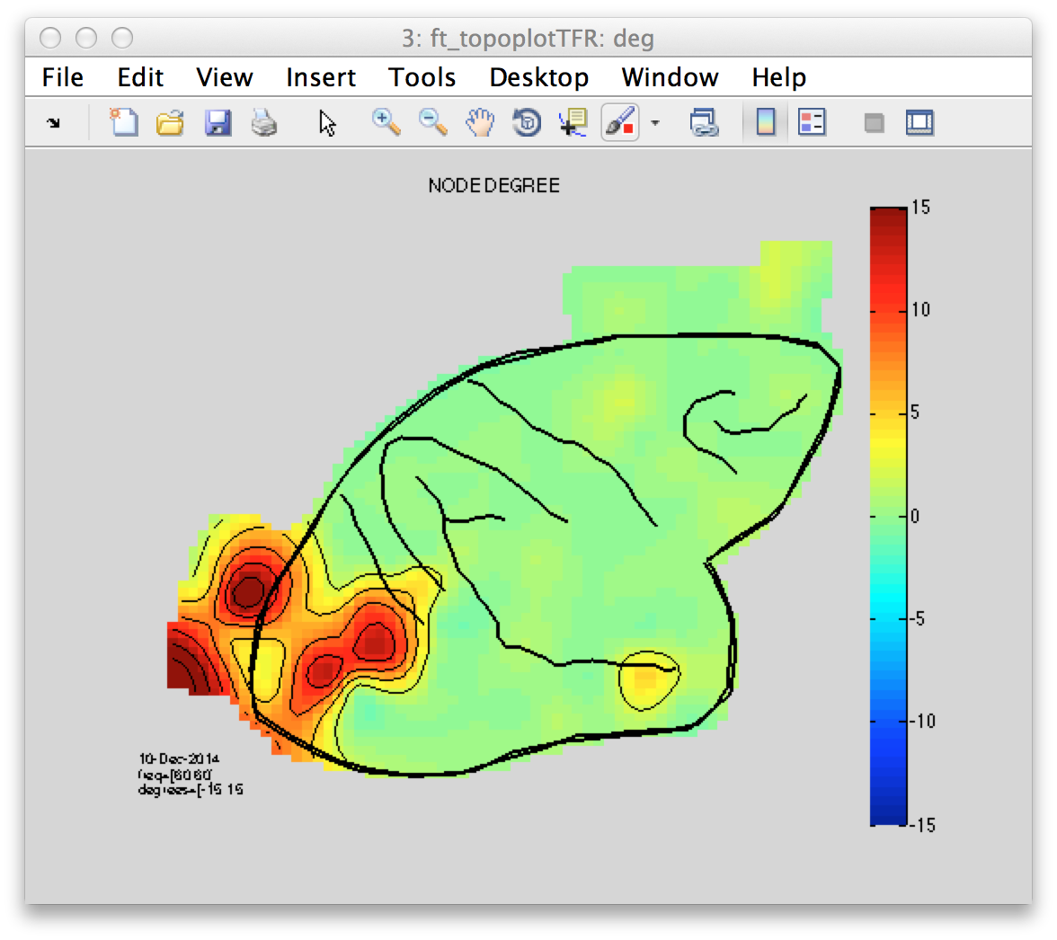
Finally, we use ft_networkanalysis to illustrate a rather formal description of the connectivity pattern in the form of a graph.
% calculate graph theoretical metric
fn=fieldnames(conn);
parameter = 'degrees';
cfg           = [];
cfg.method    = parameter;
cfg.parameter = fn{3};
cfg.threshold = .1;
deg = ft_networkanalysis(cfg, conn);

% plot the result
cfg             = [];
cfg.layout      = lay;
cfg.colormap    = 'jet';
cfg.parameter   = parameter;
cfg.zlim        = [-15 15];
cfg.colorbar    = 'yes';
cfg.interactive = 'no';
cfg.marker      = 'off';
figure;
ft_topoplotTFR(cfg, deg);
title('NODE DEGREE')
Figure 8: Node degree topography illustrating the amount of connections of a given electrode(node) to all other possible electrodes(nodes).
Summary and conclusion
This tutorial demonstrated various analysis steps associated with an evaluation of electrocorticographic recordings.
First, the data has been organized in a FieldTrip appropriate format. Psychophysiological data is often represented over various recording sites. Accordingly, data exploration is often aided by a “map” with positions corresponding to the locations of each recording site. In the context of invasive recordings it is often the case that at least a photograph capturing the implanted grid array is available. This information can be used to construct an electrode layout essential for data exploration.
Subsequently, the data has been further evaluated by decomposing the linear superposition of activity using independent components by means of ICA. On the basis of the topographic layout and the component time courses the spatial and temporal characteristics of the data had been evaluated.
Next, the spectral characteristic in the data were evaluated. It is well documented that in experimental context such as the present, i.e. visual stimulation with gratings characterized by high spatial frequency, a prominent stimulus induced power modulation in the gamma frequency range ~60 Hz is observed. The evaluated data set confirmed this observation demonstrating a prominent increase in high frequency activity. This increase was most prominent over visual areas. Following the steps described above it was possible to conclude that stimulus presentation is associated with specific brain activity characterized by time (0-2 sec post stim), frequency (~60Hz) and space (visual) “bounderies”.
Given this knowledge often we seek to characterize some quantity of interaction or connectivity between brain structures in this case electrodes. This tutorial applied “coherence” as method of choice although there are various, equally valid other methods implemented in FieldTrip. Descriptively, using a reference electrode (seed) defined as the maximal gamma band power it could be demonstrated that the propagation of the observed stimulus induced brain response is rather spatially constrained to several nearby electrodes surrounding the seed region.
Finally, a graph theoretical approach has been applied to formally describe one fundamental property of a node (electrode) in a graph (set of electrodes)- the node degree. This metric essentially describes an aspect of a network topology- the amount of connections of a given node to all possible nodes in the graph. The interpretation of the results however are often not straight forward and require an appropriate statistical contrast, which is not covered in this tutorial.
Several analysis strategies were applied but not explained in further detail. If you are unclear on the organization of the data structure suitable for analysis in FieldTrip please have a look at this FAQ. When performing frequency analysis, parameter such as length of the time window, desired and given frequency resolution etc. are very important. What is the basis for these decisions is not covered by this tutorial. If you are interested in detailed explanations of the motivation behind such decisions please evaluate the time-frequency tutorial. If you are interested in creating your own electrode layout you can consult the layout tutorial. If you are interested in a different connectivity analysis that goes somewhat beyond correlation, you can continue with the connectivity analysis tutorial.
Suggested further reading
You can read more about other types of intracranial recordings such as spike train recordings and spikes and local field potentials in the respective tutorials.
Here is also a list of related documentation:
FAQs on connectivity
FAQs on frequency analysis
- Does it make sense to subtract the ERP prior to time frequency analysis, to distinguish evoked from induced power?
- How can I do time-frequency analysis on continuous data?
- How can I test whether a behavioral measure is phasic?
- In what way can frequency domain data be represented in FieldTrip?
- How does MTMCONVOL work?
- What are the differences between the old and the new implementation of 'mtmconvol' in ft_freqanalyis?
- What are the differences between the old and the new implementation of 'mtmftt' in ft_freqanalyis?
- What are the differences between the old and the new implementation of 'wavelet' (formerly 'wltconvol') in ft_freqanalyis?
- What convention is used to define absolute phase in 'mtmconvol', 'wavelet' and 'mtmfft'?
- What does "padding not sufficient for requested frequency resolution" mean?
- What kind of filters can I apply to my data?
- Why am I not getting integer frequencies?
- Why does my output.freq not match my cfg.foi when using 'mtmconvol' in ft_freqanalyis?
- Why does my output.freq not match my cfg.foi when using 'mtmfft' in ft_freqanalyis
- Why does my output.freq not match my cfg.foi when using 'wavelet' (formerly 'wltconvol') in ft_freqanalyis?
- Why does my TFR contain NaNs?
- Why does my TFR look strange (part I, demeaning)?
- Why does my TFR look strange (part II, detrending)?
- Why is the largest peak in the spectrum at the frequency which is 1/segment length?
FAQs on data formats
- How can I append the files of two separate recordings?
- What dataformats are supported?
- How are the various MATLAB data structures defined?
- How can I convert an anatomical MRI from DICOM into CTF format?
- How can I convert one dataformat into an other?
- How can I extend the reading functions with a new dataformat?
- How can I import my own data format?
- How can I merge two datasets that were acquired simultaneously with different amplifiers?
- I have problems reading in neuroscan .cnt files. How can I fix this?
- Reading is slow, can I write my raw data to a more efficient file format?

