workshop / nigeria2025 / frequency /
Frequency analysis of resting state EEG data
General introduction
In this tutorial we will compute and compare power spectra for EEG data recorded during a resting-state experiment in which a pharmaceutical intervention was used. Before starting with this tutorial, please read through the linked description of the dataset.
The general procedure for frequency analysis on resting state data is to read the data, segment it into shorter trials or snippets, optimally using some overlap, and to compute the averaged powerspectra over all those segments. We can use different length of the trials or snippets to influence the spectral resolution, and we can use different tapering methods to influence the spectral smoothing.
Procedure
We will start by looking at the baseline session from participant 22. As it is a resting state recording, we assume that the power spectrum is stationary (i.e., constant) over time, hence we will only look at the power spectrum in the frequency domain, averaged for the whole duration of the recording, not how it changes over times.
In general the procedure consists of the following steps.
- read the continuous data using ft_preprocessing
- segment the continuous data into short snippets using ft_redefinetrial
- remove artifacts using ft_rejectartifact
- compute the averaged power spectrum using ft_freqanalysis
Reading the continuous EEG data from disk
Here we will skip the preprocessing and start directly with the preprocessed data.
clear all, close all, clc
load data_rest.mat
We can check the data that was read in memory in the MATLAB Workspace panel or by typing whos. There are four data structures corresponding to the experimental blocks.
whos

    base      1x1              68814442  struct
    mild      1x1              76362946  struct
    mode      1x1              75901106  struct
    reco      1x1              74477378  struct
Each of these is a FieldTrip data structure with a continuous segment of EEG data
disp(base)

           hdr: [1x1 struct]
       fsample: 250
    sampleinfo: [1 90000]
         trial: {[91x90000 double]}
          time: {[0 0.0040 0.0080 0.0120 ... ] (1x90000 double)}
         label: {91x1 cell}
           cfg: [1x1 struct]
          elec: [1x1 struct]
There are 90000 samples, which at 250 Hz sampling rate means that this data is 90000/250=360 seconds long, which is 6 minutes.
Effect of the window length
Taking the baseline sedation EEG data of participant 22, we will use ft_redefinetrial to cut shorter trials out of the continuous data. Specifically, we will cut the data into non-overlapping segments of various lengths (1 sec, 2 secs and 4 secs) and we will compute the power spectrum of all data segments and average them.
You can also use ft_redefinetrial to cut the data into timewindows with some overlap (e.g.. 50%). This basically implements Welsh’s method for spectral estimation.
cfg = [];
cfg.length  = 1;
cfg.overlap = 0;
base_rpt1    = ft_redefinetrial(cfg, base);

cfg.length  = 2;
base_rpt2    = ft_redefinetrial(cfg, base);

cfg.length  = 4;
base_rpt4    = ft_redefinetrial(cfg, base);
Now we use ft_freqanalysis to compute the power spectra using a boxcar window.
cfg = [];
cfg.output  = 'pow';
cfg.channel = 'all';
cfg.method  = 'mtmfft';
cfg.taper   = 'boxcar';
cfg.foi     = 0.5:1:45; % 1/cfg.length  = 1;
base_freq1  = ft_freqanalysis(cfg, base_rpt1);

cfg.foi     = 0.5:0.5:45; % 1/cfg.length  = 2;
base_freq2  = ft_freqanalysis(cfg, base_rpt2);

cfg.foi     = 0.5:0.25:45; % 1/cfg.length  = 4;
base_freq4  = ft_freqanalysis(cfg, base_rpt4);
We can plot the power spectra of channel 61 using the standard MATLAB plot function.
figure;
hold on;
plot(base_freq1.freq, base_freq1.powspctrm(61,:))
plot(base_freq2.freq, base_freq2.powspctrm(61,:))
plot(base_freq4.freq, base_freq4.powspctrm(61,:))
legend('1 sec window','2 sec window','4 sec window')
xlabel('Frequency (Hz)');
ylabel('absolute power (uV^2)');
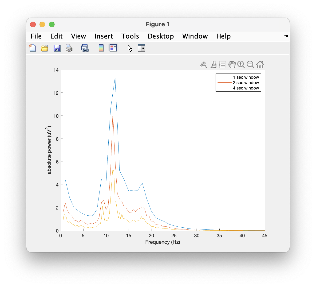
Note the differences in power and in frequency resolution for each window length.
Can you explain why the amplitude of the power spectra decrease with an increase in the window length?
Effect of different tapers
Finally, we will look at the effect of different tapers on the power estimates. To enhance the effects of the tapers, we will use the data chopped in windows of 4 seconds. So let us run again ft_freqanalysis but this time using different tapers: boxcar, Hanning and discrete prolate spheroidal sequences (DPSS, i.e., multitapers).
But before doing anything, let us recapitulate what multitapers are good for? Multitapers are typically used to achieve better control over the frequency smoothing. More tapers for a given time window will result in greater smoothing. High frequency smoothing is particularly advantageous when dealing with electrophysiological brain signals above 30 Hz. Oscillatory gamma activity (30-100 Hz) is quite broad band and thus analysis of such signals benefit from multitapering. For signals lower than 30 Hz it is recommend to use only a single taper, e.g., a Hanning taper as shown above. Beware that in the example below multitapers are used to analyze low frequencies, because there are no gamma band effects in this particular dataset.
Spectral analysis with on multitapers is done with the function ft_freqanalysis. The function uses the time in which the data has been segmented during preprocessing. Prior to the Fourier transformations, the data are “tapered”. A single taper can be applied (e.g. Hanning) or several orthogonal tapers might be used for each time window (e.g. DPSS). The power is calculated for each tapered data segment and then averaged over tapers. In the example below we already have the data segmented in windows of different sizes (1, 2, 4 seconds) and we can compute the power spectra using the following parameters:
The cfg.foi option determines the frequencies of interest, here from 1 Hz to 30 Hz in steps of 2 Hz. The step size could be decreased at the expense of computation time and redundancy.
The cfg.tapsmofrq option determines the width of frequency smoothing in Hz (= fw). We have chosen cfg.tapsmofrq = 4, which assumes a bandwidth of 8Hz smoothing (±4). For less smoothing you can specify smaller values, however, the following relation determined by the Shannon number must hold (see Percival and Walden (1993)): K = 2*tw*fw-1, where K is required to be larger than 0. K is the number of tapers applied; the more, the greater the smoothing.
cfg = [];
cfg.output    = 'pow';
cfg.channel   = 'all';
cfg.method    = 'mtmfft';
cfg.taper     = 'boxcar';
cfg.foi       = 0.5:0.25:45;
base_freq_b   = ft_freqanalysis(cfg, base_rpt4);

cfg.taper     = 'hanning';
base_freq_h   = ft_freqanalysis(cfg, base_rpt4);

cfg.taper     = 'dpss'; % here the multitapers
cfg.tapsmofrq = 4;
base_freq_d   = ft_freqanalysis(cfg, base_rpt4);

figure; hold on
plot(base_freq_b.freq, base_freq_b.powspctrm(61,:))
plot(base_freq_h.freq, base_freq_h.powspctrm(61,:))
plot(base_freq_d.freq, base_freq_d.powspctrm(61,:))
legend('4 sec boxcar', '4 secs hanning', '4 sec dpss');
xlabel('Frequency (Hz)');
ylabel('absolute power (uV^2)');
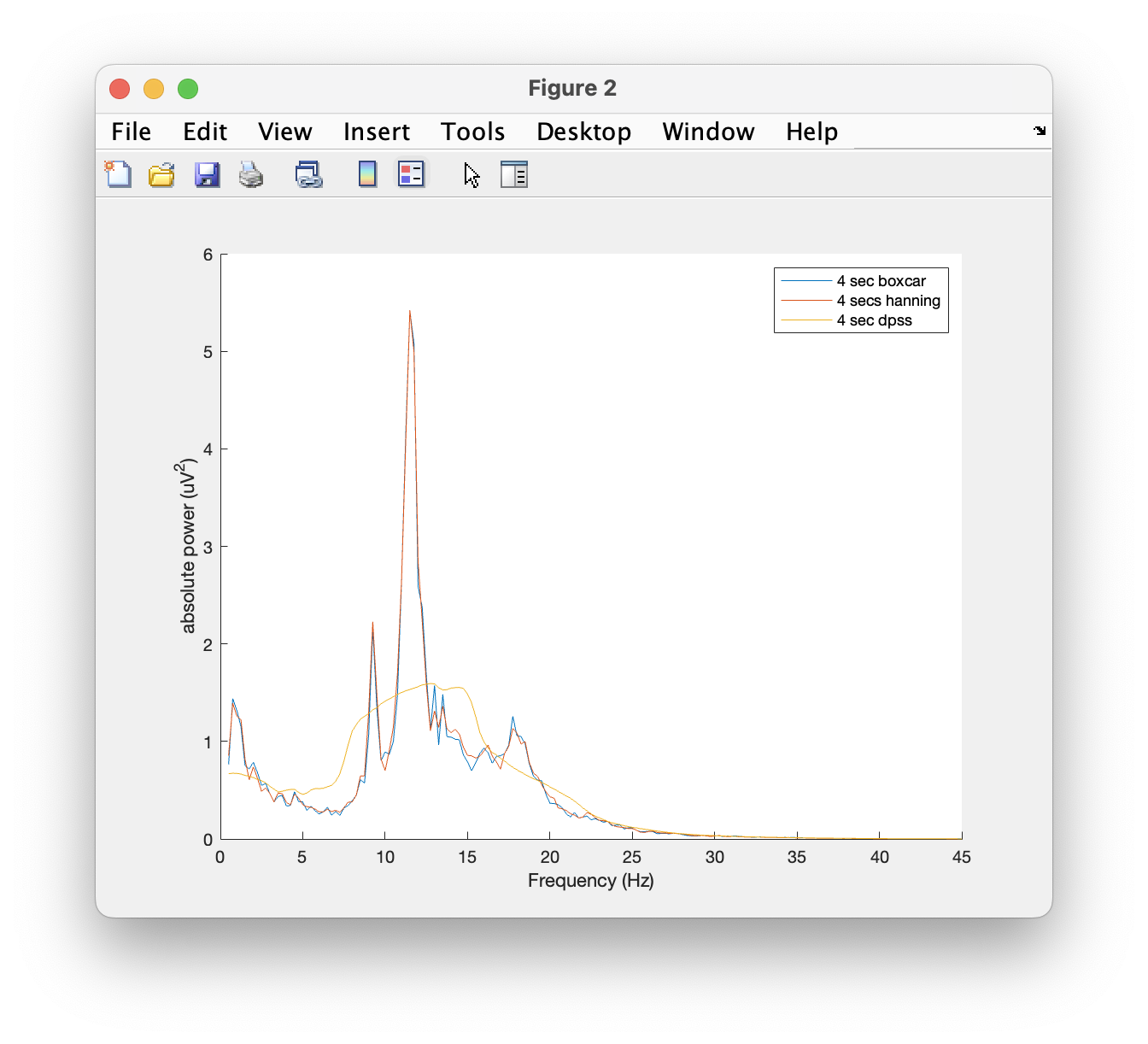
Note the differences in amplitude and frequency resolution for each taper, specially the DPSS. Can you explain why the amplitude of the power spectra decrease that much given that in this case the non-stationarity of the data is the same across tapers?
Changes in power due to propofol sedation
Finally, we will apply what we just learned to investigate the experimental effect of propofol on the resting-state EEG power spectrum.
cfg = [];
cfg.length  = 4;
cfg.overlap = 0;
base_rpt4 = ft_redefinetrial(cfg, base);
mild_rpt4 = ft_redefinetrial(cfg, mild);
mode_rpt4 = ft_redefinetrial(cfg, mode);
reco_rpt4 = ft_redefinetrial(cfg, reco);

cfg = [];
cfg.output    = 'pow';
cfg.channel   = 'all';
cfg.method    = 'mtmfft';
cfg.taper     = 'boxcar';
cfg.foi       = 0.5:0.25:45;
base_freq_b   = ft_freqanalysis(cfg, base_rpt4);
mild_freq_b   = ft_freqanalysis(cfg, mild_rpt4);
mode_freq_b   = ft_freqanalysis(cfg, mode_rpt4);
reco_freq_b   = ft_freqanalysis(cfg, reco_rpt4);

cfg.taper     = 'hanning'; % change the taper, keep the rest
base_freq_h   = ft_freqanalysis(cfg, base_rpt4);
mild_freq_h   = ft_freqanalysis(cfg, mild_rpt4);
mode_freq_h   = ft_freqanalysis(cfg, mode_rpt4);
reco_freq_h   = ft_freqanalysis(cfg, reco_rpt4);

cfg.taper     = 'dpss'; % change the taper, keep the rest
cfg.tapsmofrq = 4;
base_freq_d   = ft_freqanalysis(cfg, base_rpt4);
mild_freq_d   = ft_freqanalysis(cfg, mild_rpt4);
mode_freq_d   = ft_freqanalysis(cfg, mode_rpt4);
reco_freq_d   = ft_freqanalysis(cfg, reco_rpt4);

cfg = [];
cfg.layout = 'GSN-HydroCel-128';
cfg.showscale = 'no';
cfg.showcmnt = 'no';

figure; ft_multiplotER(cfg, base_freq_b, mild_freq_b, mode_freq_b, reco_freq_b)
figure; ft_multiplotER(cfg, base_freq_h, mild_freq_h, mode_freq_h, reco_freq_h)
figure; ft_multiplotER(cfg, base_freq_d, mild_freq_d, mode_freq_d, reco_freq_d)
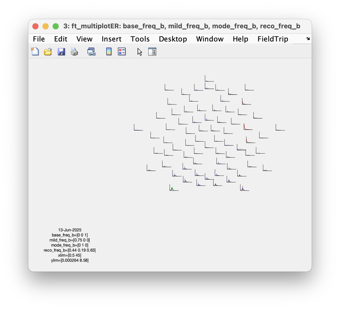
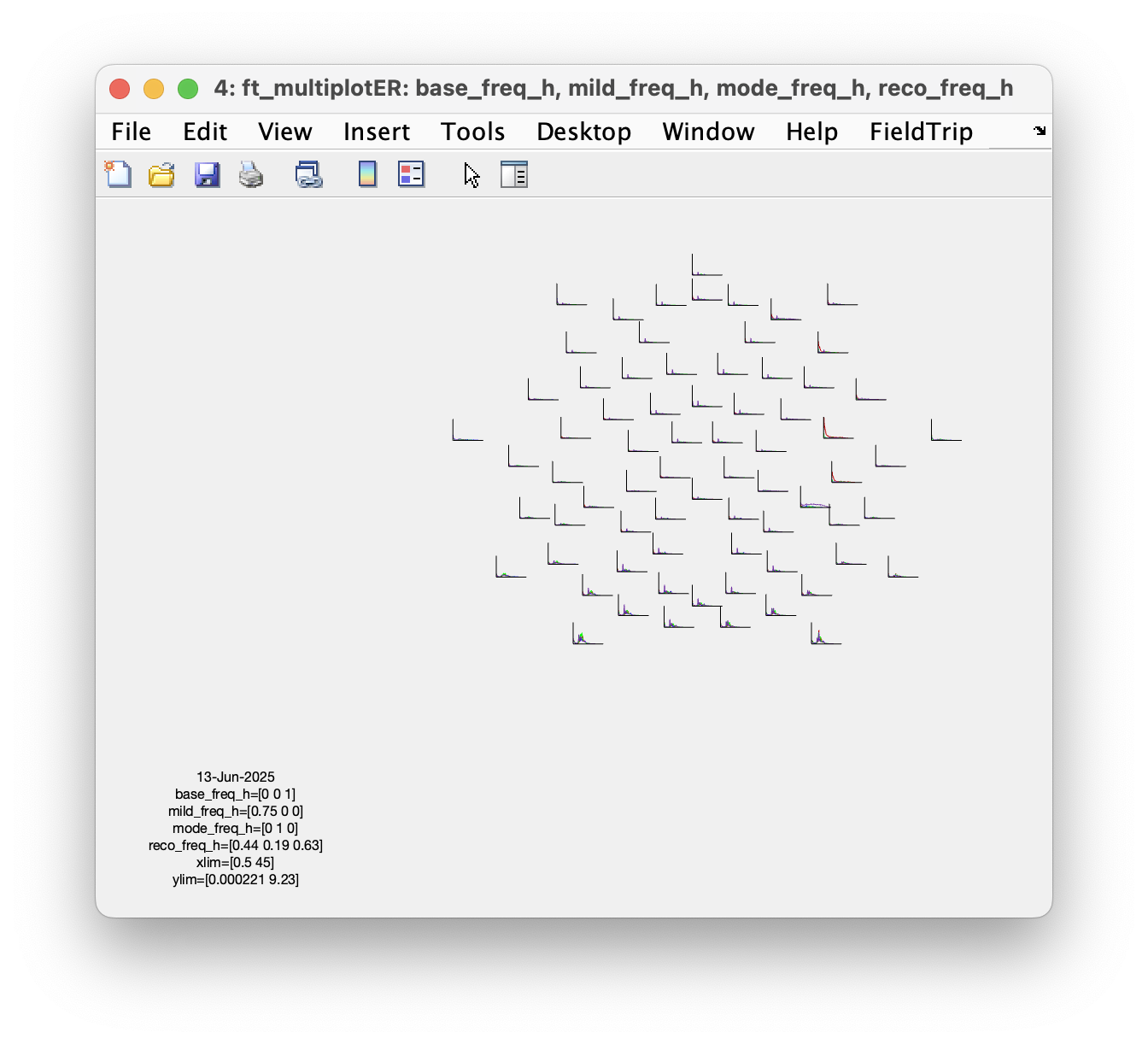
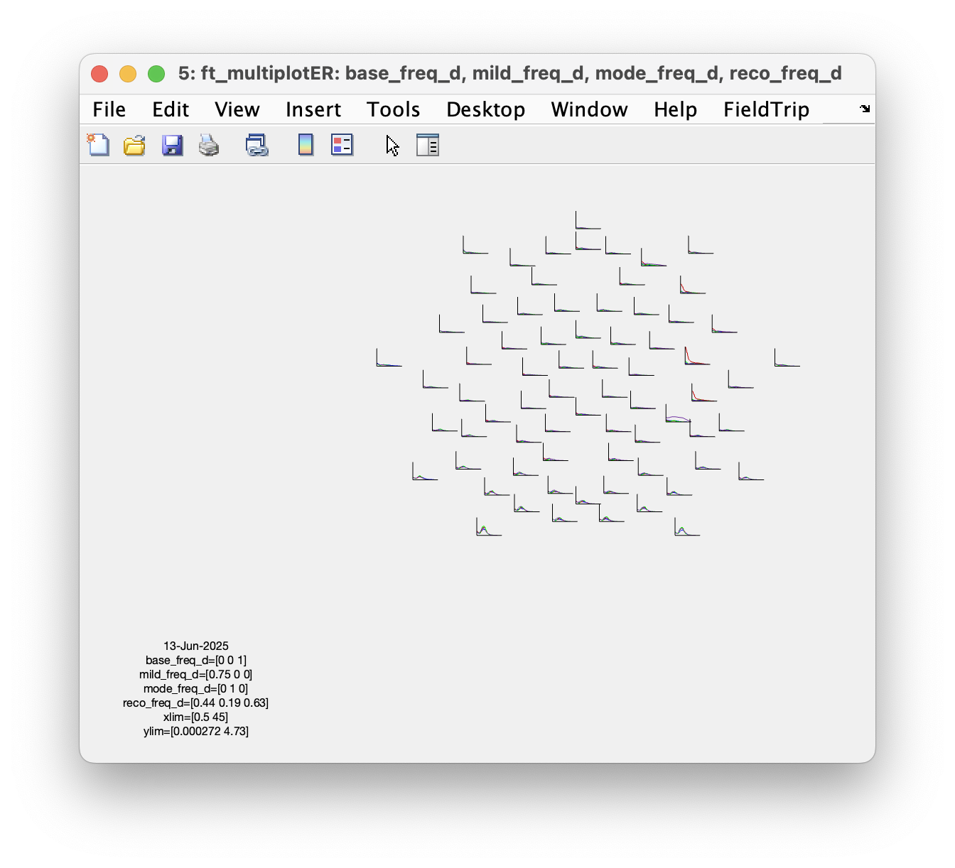
Which set of parameters is more sensitive to detect the shift of low-beta power?
Time-frequency analysis on continuous data
Although often we assume stationarity of the data in a resting-state experiment, it is possible to look at how the power spectrum changes over time. For that we are using this trick.
As before, we compute the power spectrum on the segmented data, but now we specify cfg.keeptrials='yes' to prevent the trials from being averaged.
cfg = [];
cfg.output      = 'pow';
cfg.channel     = 'all';
cfg.method      = 'mtmfft';
cfg.taper       = 'dpss';
cfg.tapsmofrq   = 1;
cfg.keeptrials  = 'yes';
cfg.foi         = 0.5:0.25:45;
base_freqtrials = ft_freqanalysis(cfg, base_rpt4);

disp(base_freqtrials)
The output has a power spectrum for each channel and each trial. We can go back to the original data and compute the middle of the 4-second windows, so that we know the latency of each trial in the experimental block (from 0 to 360 seconds).
begsample = base_rpt4.sampleinfo(:,1);
endsample = base_rpt4.sampleinfo(:,2);
time = ((begsample+endsample)/2) / base_rpt4.fsample;
This gives us a vector that we can use as the time axis, with one latency per trial. The first trial goes from 0 to 4 seconds, so we assign that the latency 2. The second trial goes from 4 to 8, so we assign that the latency 6. Etcetera.
Note that this is different from a more conventional time-frequency analysis, where we use the peri-stimulus time axis to get a much higher resolution time-frequency representation, for example using wavelet analysis. That is presented elsewhere, for example in the time-frequency analysis tutorial.
Now we can re-shuffle the power spectrum to change it into a representation similar to that of the time-frequency analysis. The trial dimension in the data becomes the time dimension, and we add the time axis.
base_timefreq           = base_freqtrials;
base_timefreq.powspctrm = permute(base_freqtrials.powspctrm, [2, 3, 1]);
base_timefreq.dimord    = 'chan_freq_time'; % it used to be 'rpt_chan_freq'
base_timefreq.time      = time;             % add the description of the time dimension

cfg = [];
cfg.baselinetype = 'db';
cfg.baseline = [-inf inf];
cfg.layout = 'GSN-HydroCel-128';
cfg.showscale = 'no';
cfg.showcmnt = 'no';
ft_multiplotTFR(cfg, base_timefreq);