workshop / oslo2019 / beamforming /
Beamforming oscillatory responses in MEG data
Introduction
This tutorial explains beamformer source reconstruction techniques in the frequency domain. You will learn how to compute appropriate time-frequency windows, how to apply the spatial filter, and about options for contrasting the effect of interest against some control/baseline. Finally, you will be guided through different options to visualize the results overlaid on a structural MRI.
For this, we will continue working on the paradigm we used in the previous tutorial. However, we will do the source reconstruction using the MEG data recorded in the same session, not the EEG data. Please note that later in this workshop you will learn how to construct a forward model, so details on that step are omitted here. The forward modeling lecture will be geared towards EEG, so that you can apply what you learn here also to EEG data.
This tutorial contains the hands-on material for the Oslo 2019 workshop and is complemented by this lecture, which was filmed at an earlier workshop at NatMEG.
Background
In the Time-Frequency Analysis tutorial, we identified strong oscillations in the beta band in a motor response paradigm. The goal of this tutorial is to identify the sources responsible for producing this oscillatory activity. We will apply the beamformer technique: this is a spatially adaptive filter, allowing us to estimate the amount of activity at any given location in the brain. The inverse filter is based on minimizing the source power (or variance) at a given location, subject to the ‘unit-gain constraint’. This latter part means that, if a source had power of amplitude 1 and was projected to the sensors by the leadfield, the inverse filter applied to the sensors would reconstruct amplitude 1 at that location. Beamforming assumes that sources in different parts of the brain are not temporally correlated.
For beamforming, the brain is divided in a regular 3D grid and the source strength for each grid point is computed. The method applied here is termed Dynamical Imaging of Coherent Sources (DICS) and the estimates are calculated in the frequency domain (Gross et al. 2001). Other beamformer methods estimate source activity in the time domain, e.g., the Linearly Constrained Minimum Variance (LCMV) and the Synthetic Aperture Magnetometry (SAM) methods (van Veen et al., 1997; Robinson and Cheyne, 1997). All of these methods can produce a 3D spatial distribution of source power. This distribution is then overlaid on a structural image of the subject’s brain. Furthermore, these distributions of source power can be subjected to statistical analysis. It is ideal to contrast the activity of interest against an explicit control or baseline activity. Options for this will be discussed below, but it is best to keep this in mind when designing your experiment from the start, rather than struggle to find a suitable control/baseline after data collection.
This tutorial does not cover forward model computation. We will load the needed ingredients for this from disk. However, there will be a forward modeling tutorial at a later stage of this workshop.
Procedure
- Load the forward model including the headmodel, sourcemodel, and leadfield matrix (for computation of the forward model see here)
- Load the data from disk and define the period of interest using ft_redefinetrial
- Compute the cross-spectral density matrix for all MEG channels using the function ft_freqanalysis
- Compute a spatial filter and estimate the power of the sources using ft_sourceanalysis
- Visualize the result with ft_sourceplot
- Compute a common spatial filter to difference two conditions
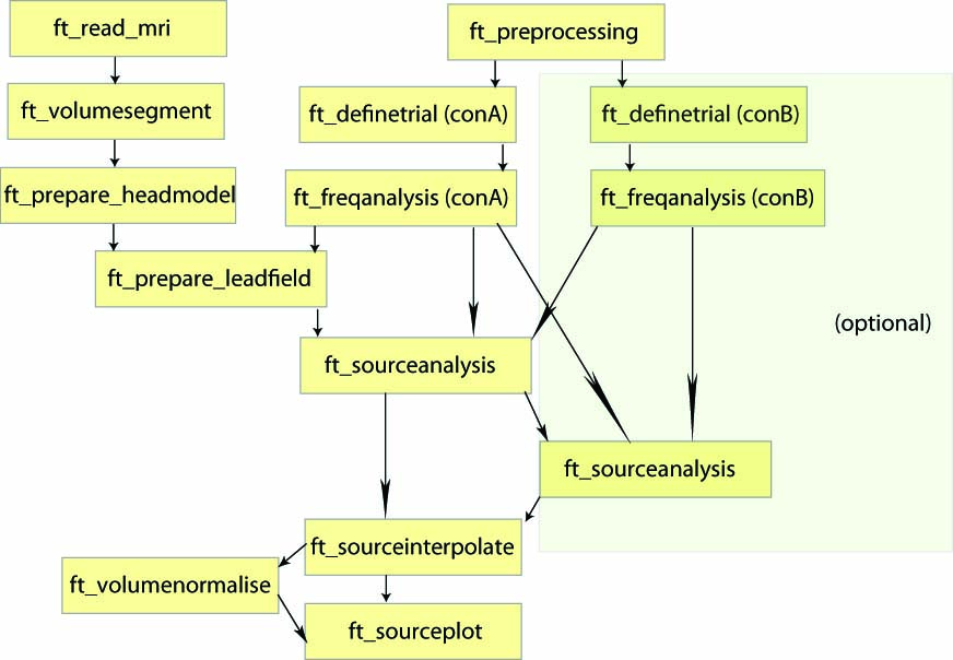
Figure: An example of a pipeline to locate oscillatory sources.
Preparing the data
Loading the data
First, we are going to load the MEG data, which has already been preprocessed very similarly to what you learned in the Introduction tutorial.
Load the data using the following command:
load data_clean_MEG_responselocked.mat
Loading the ingredients of the forward model
The first requirement for source reconstruction is a forward model. The forward model allows us to calculate the distribution of the magnetic field on the MEG sensors given a hypothetical current distribution. We will learn more about that in the Forward modeling tutorial tomorrow. Here, we will skip this step and load all the ingredients from disk.
We load the precomputed headmodel that described the geometry and conductive properties of the head, and the sourcemodel that describes both information about the assumed source locations in our forward model, as well as the leadfield matrix for each source. The leadfield matrix describes the magnetic field of a source at specific location, i.e. it represents the visibility of that source on the sensors.
load headmodel_meg.mat
load sourcemodel
Plotting the forward model
It is always a good idea to plot all ingredients of the forward model together, to see if they line up. So here we plot the grid with source positions, the headmodel, and the sensor positions together:
figure
hold on
inside_idx = find(sourcemodel.inside);  % find grid points inside the brain

% plot the grid points:
plot3(sourcemodel.pos(inside_idx, 1), sourcemodel.pos(inside_idx, 2), ...
    sourcemodel.pos(inside_idx, 3), ...
    'k.', 'markersize', 20)

% plot the headmodel:
ft_plot_headmodel(headmodel_meg, 'facealpha', 0.1, ...
    'facecolor', 'brain', 'edgecolor', 'brain', 'edgealpha', 0.1)

% plot the sensors:
plot3(data_clean_MEG_responselocked.grad.chanpos(:, 1), ...
    data_clean_MEG_responselocked.grad.chanpos(:, 2), ...
    data_clean_MEG_responselocked.grad.chanpos(:, 3), ...
    'b*', 'markersize', 20);

view(90, 0)
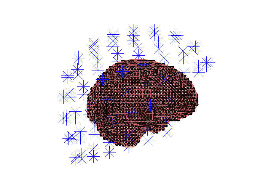
Figure: The different parts for the forward model all line up.
Identifying a time window of interest
We want to identify the sources of the oscillatory activity in the beta band. We have identified 18 Hz as the center frequency of the beta activity. We first use ft_redefinetrial to extract the relevant time window from the complete trials. Remember, that it is important that the length of the time window matches with an integer number of oscillatory cycles. Here 9 cycles are used, resulting in a 9/18 Hz = 0.5 s time window. Thus, the time window we will use ranges from 0.35 to 0.85 second after response onset (see Figure 2).
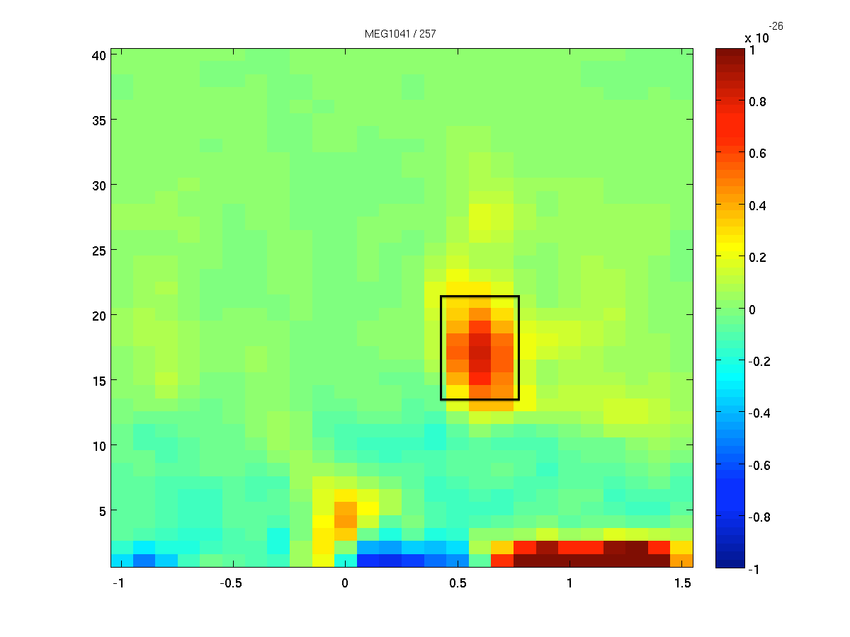
Figure: The time-frequency presentation used to determine the time- and frequency-windows prior to beamforming.
Now we select the time window of interest using ft_redefinetrial.
% Select time window of interest
cfg = [];
cfg.toilim = [0.35 0.85];
data_timewindow = ft_redefinetrial(cfg, data_clean_MEG_responselocked);
Exercise 1: data length
Why is it important that the length of each data piece is the length of a fixed number of oscillatory cycles?
Calculating the cross spectral density matrix
The beamformer is based on an adaptive spatial filter. For the DICS method, the spatial filter is derived from the frequency counterpart of the covariance matrix: the cross-spectral density matrix. This matrix contains the cross-spectral densities for all sensor combinations and is computed from the Fourier transformed data of the single trials. It is given as output when cfg.output = 'powandcsd'. The frequency of interest is 18 Hz and the smoothing window is +/- 4 Hz, which is given by using cfg.taper = 'dpss' and the taper smoothing frequency cfg.tapsmofrq = 4.
We choose to only use the trials with the left hand response for now, which is why we specify the trials corresponding to the trigger value 256 in cfg.trials.
% Frequency analysis for beamformer
cfg = [];
cfg.trials       = find(data_timewindow.trialinfo(:, 1) == 256);
cfg.channel      = {'MEG*2', 'MEG*3'};
cfg.method       = 'mtmfft';
cfg.taper        = 'dpss';
cfg.output       = 'powandcsd';
cfg.keeptrials   = 'no';
cfg.foi          = 18;
cfg.tapsmofrq    = 4;

powcsd_left      = ft_freqanalysis(cfg, data_timewindow);
The cross-spectral density data structure has a similar data structure as other output of ft_freqanalysis:
powcsd_left =

      label: {204x1 cell}     % Channel labels
     dimord: 'chan_freq'      % Dimensions in the data
       freq: 17.8571          % Target frequency
  powspctrm: [204x1 double]   % Power spectrum
   labelcmb: {20706x2 cell}   % Channel combinations
  crsspctrm: [20706x1 double] % Cross-spectral density matrix
       elec: [1x1 struct]     % EEG electrode information
       grad: [1x1 struct]     % MEG sensor information
        cfg: [1x1 struct]     % Configuration
How come our target frequency is 17.8571, didn’t we ask for 18? Hint: How large is our time window?
MEG source analysis on the left hand reaction
Using the cross-spectral density and the leadfield matrices that we loaded, a spatial filter is calculated for each grid point. By applying the filter to the Fourier transformed data, we can estimate the power for the left hand reaction activity. This results in a power estimate for each grid point.
cfg              = [];
cfg.method       = 'dics';
cfg.sourcemodel  = sourcemodel;
cfg.headmodel    = headmodel_meg;
cfg.channel      = {'MEG*2', 'MEG*3'};
cfg.frequency    = 18;
cfg.senstype     = 'MEG'; % Must be 'MEG', although we only kept MEG channels,
                          % information on EEG channels is still present in data
cfg.dics.projectnoise = 'yes';
cfg.dics.lambda  = '5%';
source_left = ft_sourceanalysis(cfg, powcsd_left);
The source data structure has the following fields:
source_left =

  freq: 17.8571           % Target frequency
   dim: [26 36 28]        % Dimensions of the data
inside: [26208x1 logical] % Positions that are inside the brain volume
   pos: [26208x3 double]  % 3-D Coordinates of grid points
method: 'average'         % Operation applied over trials
   avg: [1x1 struct]      % Average power for each point in the source estimate
   cfg: [1x1 struct]      % Configuration
Interpolate the results on the MRI for plotting
The grid of estimated power values can be plotted superimposed on the anatomical MRI. This requires the output of ft_sourceanalysis to match the position of the MRI. The function ft_sourceinterpolate interpolates the relatively low-resolution source level estimates on the high-resolution structural MRI. We only need to specify what parameter we want to interpolate and to input the MRI we want to use for interpolation.
First, we will load the MRI. It is important that you use the MRI that was realigned with the sensors, or your source activity data will not match the anatomical data.
load mri_realigned2.mat
Before interpolating the source activity we will reslice the MRI using ft_volumereslice. The consequence of reslicing is that the size of the MRI is decreased (it is rather large now) and the output voxels are nicely aligned with the x, y, and z-axes, so that the image is plotted correctly. See also this frequently asked question.
mri_resliced = ft_volumereslice([], mri_realigned2);
Now we can interpolate the estimated source activity onto the voxels of the MRI:
cfg            = [];
cfg.parameter = 'pow';
source_left_int  = ft_sourceinterpolate(cfg, source_left, mri_resliced);
And now, we can plot the interpolated data:
cfg = [];
cfg.method        = 'ortho';
cfg.funparameter  = 'pow';
cfg.funcolorlim   = 'maxabs';
cfg.opacitymap    = 'rampup';

ft_sourceplot(cfg, source_left_int);
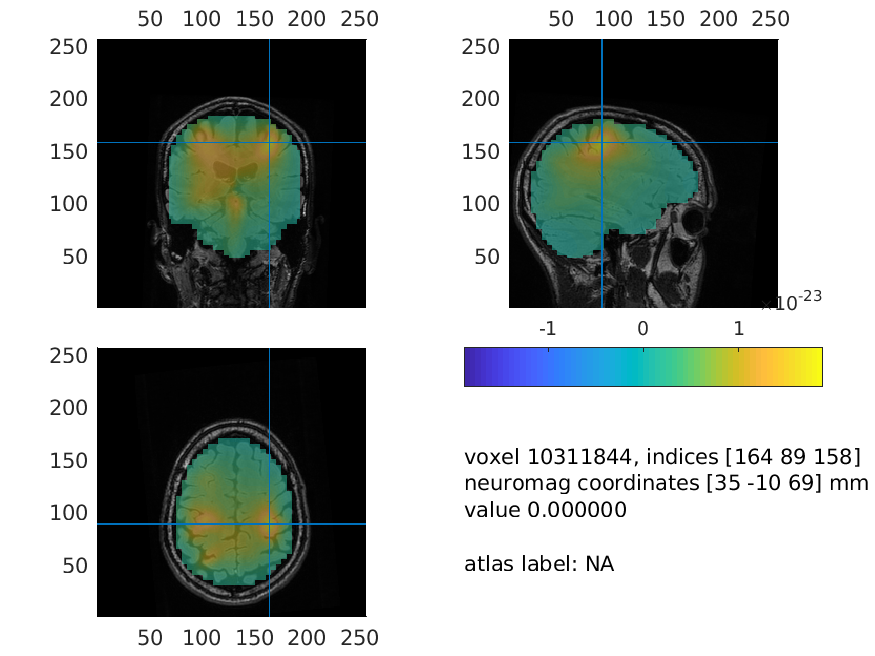
Figure: Source reconstructed oscillatory power of the beta response in the left-hand condition.
Bonus: Source analysis for contrasting conditions
It is ideal to contrast the activity of interest against some control.
- Suitable control windows are, for example:
- Activity contrasted with baseline (example not shown)
- Activity of condition 1 contrasted with condition 2 (example shown here, using left vs right)
- However, if no other suitable data condition or baseline time-window exists, then
- Use normalized leadfields (that is what we did above!)
- Activity contrasted with estimated noise
Why shouldn’t we calculate a spatial filter for both conditions separately in the case of contrasting conditions? Would there be a reason to do so?
The statistical null hypothesis for both options within (1) is that the data are the same in both conditions, and thus the best spatial filter would be the one that is computed using both data conditions together (also known as ‘common filters’). This common filter is then applied separately to each condition. To calculate the common filter, we will use the extracted time window, pooled over both conditions.
Frequency analysis for both conditions
To start with this, we need to compute the oscillatory power for both conditions alone (we already did that for the left hand trials above!) and for both conditions together.
cfg = [];
cfg.channel      = {'MEG*2', 'MEG*3'};
cfg.method       = 'mtmfft';
cfg.taper        = 'dpss';
cfg.output       = 'powandcsd';
cfg.keeptrials   = 'no';
cfg.foi          = 18;
cfg.tapsmofrq    = 4;

% for common filter over conditions: use all the data
powcsd_all      = ft_freqanalysis(cfg, data_timewindow);

% for conditions: we already computed "powcsd_left", right hand trials:
cfg.trials       = find(data_timewindow.trialinfo(:,1) == 4096);
powcsd_right     = ft_freqanalysis(cfg, data_timewindow);
You could also compute powcsd_all with cfg.keeptrials set to yes and use the cfg.trials option later in ft_sourceanalysis or using ft_selectdata. This would be computationally more efficient, but requires more memory.
Compute the spatial common filter and apply it to the conditions
We now use all the data as input for computing the common spatial filter. We specify that we would like to keep the computed spatial filter in the output by setting cfg.dics.keepfilter to yes, so that way we can reuse it later.
cfg              = [];
cfg.method       = 'dics';
cfg.sourcemodel  = sourcemodel;
cfg.headmodel    = headmodel_meg;
cfg.channel      = {'MEG*2', 'MEG*3'};
cfg.frequency    = 18;
cfg.senstype     = 'MEG';
cfg.dics.projectnoise = 'yes';
cfg.dics.lambda       = '5%';
cfg.dics.keepfilter   = 'yes';  % We want to reuse the calculated filter later on

source_all = ft_sourceanalysis(cfg, powcsd_all);
To apply this common spatial filter to the trials of our two conditions separately, we run ft_sourceanalysis again - for both conditions - but specify that we want to use the filter we just computed.
cfg              = [];
cfg.method       = 'dics';
cfg.sourcemodel  = sourcemodel;
cfg.headmodel    = headmodel_meg;
cfg.channel      = {'MEG*2', 'MEG*3'};
cfg.frequency    = 18;
cfg.senstype     = 'MEG';
cfg.sourcemodel.filter = source_all.avg.filter;  % We apply the previously computed spatial filter

source_left  = ft_sourceanalysis(cfg, powcsd_left);
source_right = ft_sourceanalysis(cfg, powcsd_right);
After successfully applying the above steps, we obtained an estimate of the beta-band suppression in both experimental conditions at each grid point in the brain volume. Now we can compute the difference between the two conditions. Here we take the ratio between the two conditions, normalized by their sum. In this operation we assume that the noise bias is the same for both experimental conditions and it will thus cancel out when contrasting.
source_diff = source_left;
source_diff.avg.pow = (source_left.avg.pow - source_right.avg.pow) ./ ...
                      (source_left.avg.pow + source_right.avg.pow);
It would be better here to use ft_math to compute the contrast between the condition. It will ensure that the data is consistent (i.e. prevent accidentally combining different source locations in the two estimates for the two conditions) and it keeps the provenance consistent.
Interpolate and plot the difference between conditions
This is the same operations as we did above. We interpolate the data onto the structural MRI and then plot the result.
% interpolate:
cfg = [];
cfg.parameter = 'pow';
source_diff_int  = ft_sourceinterpolate(cfg, source_diff, mri_resliced);

% Plot the result
cfg = [];
cfg.method        = 'ortho';
cfg.funparameter  = 'pow';
cfg.funcolorlim   = 'maxabs';
cfg.opacitymap    = 'rampup';

ft_sourceplot(cfg, source_diff_int);
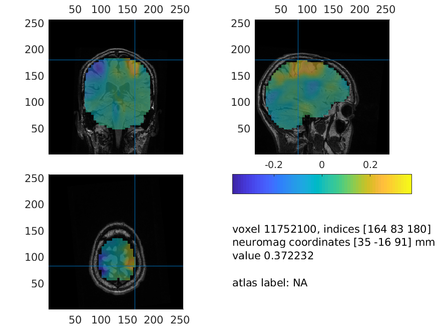
Figure: Source plot of the difference in beta power between the left and right hand response.
Exercise 2: understanding the results
Try to explain the location of the red and blue blobs.
The ‘ortho’ method is not the only plotting method implemented. Use the ‘help’ of ft_sourceplot to find what other methods there are and plot the source level results. What are the benefits and drawbacks of these plotting routines?
Exercise 3: regularization
The regularization parameter lambda was ‘5%’. Change it to ‘0%’ or to ‘10%’ and plot the power estimate. How does the regularization parameter affect the properties of the spatial filter?