Forward modeling for EEG source reconstruction

Introduction

This tutorial goes through the necessary steps for creating a robust forward model for EEG source reconstruction.

It is part of the Oslo 2019 workshop tutorials, where tutorials can be found on preprocessing and ERPs, time-frequency representations, statistics and source reconstruction.

The data for the tutorial is available here

Background

To do source reconstruction, a so-called forward model is needed. The forward model constrains the solution space for the inverse models (source reconstructions) that we may wish to apply to our data sets. If we had no constraints at all, there would be an infinite number of solutions (inverse models) that would satisfy the problem that we are trying to solve, which is: which are the latent/unobserved variables (sources) that give rise to the observed variables (the time courses observed on electrodes, i.e. the EEG data). By constraining the solution in sensible ways and applying sensible algorithms we can find a unique solution for the inverse model. In this tutorial, we will focus on constraining the solution, i.e. providing a sensible forward model. The application of sensible algorithms is the source reconstruction presented by Britta Westner yesterday.

Optimally, we have individual Magnetic Resonance Images (MRIs) available for each subject. If this is not so, it is also possible to use a template brain for source reconstruction. See here. In this tutorial we will assume that you have individual structural MRIs at your disposal.

There are four components of a forward model

1. A head model: we need to know how the electric currents generated at the source spread throughout the volume conductor (the head, containing the borders between brain and skull and between skull and skin)
2. A sensor description: we need to know where the sensors are that pick up the activity coming from the sources
3. A source model: we need to know where the sources are - preferably they should be in the brain
4. A lead field : we need to know how the sources and sensors “connect” to one another. That is, for each source (activated at unit strength (1 Am)) we calculate the electric potential vector at each sensor (electrode). It may be seen that the lead field (component 4) is really the “sum” of the information from components 1-3.

The challenge of coordinate systems

One challenge that we will face is that the source model and the head model are going to be based on the MRI data where positions are going to be expressed in the scanner’s coordinate system, whereas the sensor description is based on a another coordinate system. In our case, they were digitized using a so-called Polhemus system, where the coordinate system is centered on an x-axis which runs between the pre-auricular points on the ears of the subject. The y-axis runs through the center point of the x-axis and towards the nasion of the subject. Finally, the z-axis is perpendicular to the x- and y-axes. The three points, the pre-auricular points and the nasion are together called the fiducials.

We need to bring these two coordinate systems together before we can create a sensible forward model. The first step, however, is to read in the MRI data.

Before we begin

We will clear all variables that we have in the workspace, restore the default path, add fieldtrip and run ft_defaults

clear variables
restoredefaultpath

addpath /home/lau/matlab/fieldtrip/ %% set your own path
ft_defaults

Read in and visualize the MRI data

The anatomical MRI data available here comes directly from the scanner in the DICOM format (read more about the DICOM format here. You can download dicom.zip. Please unzip the files in a folder called dicom, which should be put in the folder where you have the other scripts used for the Oslo 2019 tutorials.

DICOM datasets consist of a large number of files, one per slice. As filename you have to specify a single file, the reading function will automatically determine which other slices are part of the same anatomical volume and put them in the correct order.

We read in the data using ft_read_mri

mri_file = './dicom/00000001.dcm';
mri = ft_read_mri(mri_file);

And plot it using ft_sourceplot with an empty cfg. This is the same function that can be used to overlay MRIs with functional data.

cfg = [];

ft_sourceplot(cfg, mri);

print -dpng original_mri.png

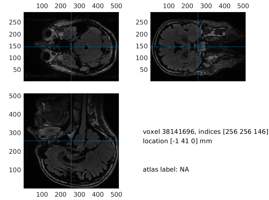
Figure 1: Plot of the original MRI

Co-register the anatomical MRI to the EEG

The next step is to bring the two coordinate systems (DICOM and Polhemus) together. Choosing interactive for cfg.method allows us to click on the fiducial points on the MR image. We choose neuromag as our coordinate system here, which has its origo at (0, 0, 40) in the coordinate system digitized by the Polhemus.

cfg          = [];
cfg.method   = 'interactive';
cfg.coordsys = 'neuromag';

mri_aligned_fiducials = ft_volumerealign(cfg, mri);

In this case, we also have extra head shape points digitized with the Polhemus system. We are going to better the co-registration using these as well. If the initial looks okay (e.g., nose points are around the MRI-nose), then just press quit, and the Iterative Closest Point algorithm do its work (cfg.headshape.icp)

load headshape.mat

cfg                     = [];
cfg.method              = 'headshape';
cfg.headshape.headshape = headshape;
cfg.headshape.icp       = 'yes'; % use iterative closest point procedure
cfg.coordsys            = 'neuromag';

mri_aligned_headshape = ft_volumerealign(cfg, mri_aligned_fiducials);

We follow this up by a check running ft_volumerealign again

ft_volumerealign(cfg, mri_aligned_headshape);

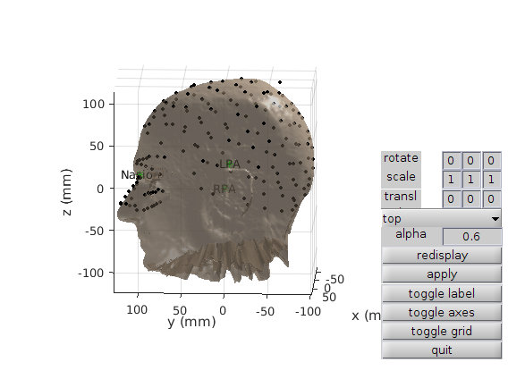
Figure 2: Plot of the co-registration after applying Iterative Closest Points on the Polhemus head shape points

load mri_aligned_headshape

Re-slice the MRI

We reslice the MRI on to a 1x1x1 mm cubic grid which is aligned with the coordinate axes. This is convenient for plotting,

cfg            = [];
cfg.resolution = 1;

mri_resliced = ft_volumereslice(cfg, mri_aligned_headshape);

and when we plot it now, the axes are more conveniently located - note that everything could have been done with the “flipped” images as well.

cfg = [];

ft_sourceplot(cfg, mri_resliced);

print -dpng mri_aligned_resliced.png

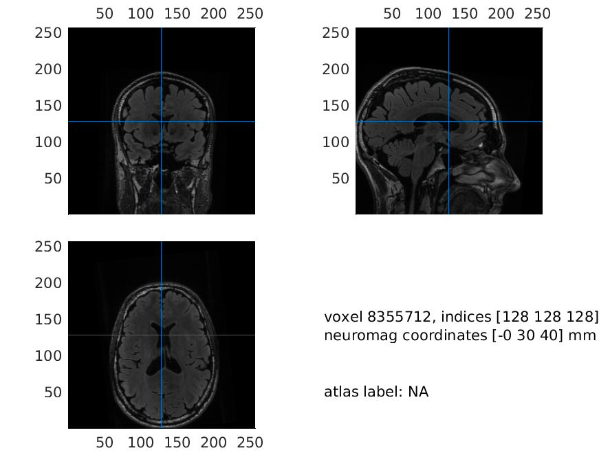
Figure 3: Plot of the resliced MRI, where axes are located in a more convenient manner

Segment the brain

The next step is to segment our coregistered and resliced MR image into the three kinds of tissues that we need to care about in our forward model for EEG data, namely the brain tissue, the skull tissue and the scalp tissue. We use ft_volumesegment for this. (This function relies on implementations from SPM)

cfg        = [];
cfg.output = {'brain' 'skull' 'scalp'};

mri_segmented = ft_volumesegment(cfg, mri_resliced);

Creating meshes

From this segmentation, we will now create a mesh for each of the three tissues.

cfg             = [];
cfg.method      = 'projectmesh';
cfg.tissue      = 'brain';
cfg.numvertices = 3000;

mesh_brain = ft_prepare_mesh(cfg, mri_segmented);
mesh_brain = ft_convert_units(mesh_brain, 'm'); % Use SI Units

cfg             = [];
cfg.method      = 'projectmesh';
cfg.tissue      = 'skull';
cfg.numvertices = 2000;

mesh_skull = ft_prepare_mesh(cfg, mri_segmented);
mesh_skull = ft_convert_units(mesh_skull, 'm'); % Use SI Units

cfg             = [];
cfg.method      = 'projectmesh';
cfg.tissue      = 'scalp';
cfg.numvertices = 1000;

mesh_scalp = ft_prepare_mesh(cfg, mri_segmented);
mesh_scalp = ft_convert_units(mesh_scalp, 'm'); % Use SI Units

mesh_eeg = [mesh_brain mesh_skull mesh_scalp];

and we will plot them

figure

ft_plot_mesh(mesh_brain, 'edgecolor', 'none', 'facecolor', 'r')
ft_plot_mesh(mesh_skull, 'edgecolor', 'none', 'facecolor', 'g')
ft_plot_mesh(mesh_scalp, 'edgecolor', 'none', 'facecolor', 'b')
alpha 0.3
view(132, 14)

print -dpng meshes.png

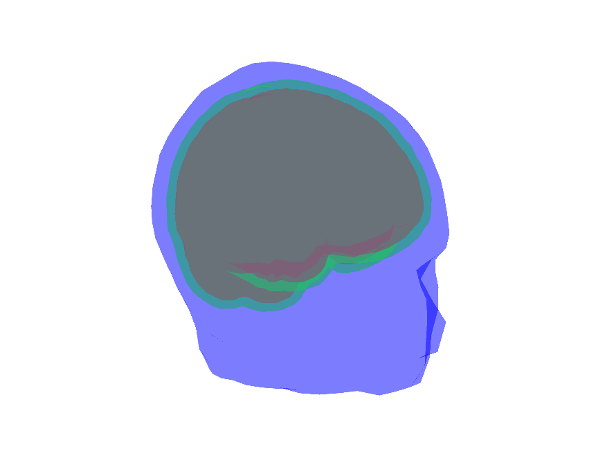
Figure 4: Plot of the three meshes (_brain, skull _and scalp)

Head models (component 1)

We will now use these non-intersecting meshes to specify the head models, which will later be used to indicate how currents spread throughout the volume conductor. We create two models, one with the bemcp method and one with the dipoli method. For the article on the dipoli method, see Oostendorp & van Oosterom, 1989 and for an article on the bemcp method, see for example Mosher et al., 1999. Do note that the dipoli method will not work on a Windows computer. The headmodel_dipoli can be downloaded here instead. The best choice is to use OpenMEEG, (cfg.method = ‘openmeeg’). This requires some manual installation and setting up, so it is not covered here.

cfg              = [];
cfg.method       = 'bemcp';
cfg.conductivity = [1 1/80 1] * (1/3); % S/m

headmodel_bem = ft_prepare_headmodel(cfg, mesh_eeg);
headmodel_bem = ft_convert_units(headmodel_bem, 'm'); % Use SI Units

cfg              = [];
cfg.method       = 'dipoli'; % will not work with Windows
cfg.conductivity = [1 1/80 1] * (1/3); % S/m

headmodel_dipoli = ft_prepare_headmodel(cfg, mesh_eeg);
headmodel_dipoli = ft_convert_units(headmodel_dipoli, 'm'); % Use SI Units

Now let’s set the headmodel that we are going to use for now, starting with headmodel_bem

headmodel = headmodel_bem;

and let’s plot it

figure
ft_plot_headmodel(headmodel, 'facealpha', 0.5)
view(90, 0)

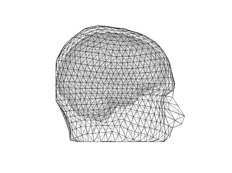
Figure 5: Plot of the head model with the three meshes (_brain, skull _and scalp). Use the zooming tools to see the differences between the different tissues.

Getting electrodes in the right position (component 2)

Now, we will load the electrodes description elec.mat that we have gotten from our Polhemus data and convert units to SI.

load elec.mat
elec = ft_convert_units(elec, 'm'); % Use SI units

and then plot them

figure
hold on
ft_plot_sens(elec, 'elecsize', 40);
ft_plot_headmodel(headmodel, 'facealpha', 0.5);
view(90, 0)

Figure 6: Some electrodes are inside the head

Realigning electrodes

We will now realign the electrodes by projecting them to the surface

% scalp indices differ for the two types of head models
if strcmp(headmodel.type, 'bemcp')
    scalp_index = 3;
elseif strcmp(headmodel.type, 'dipoli')
    scalp_index = 1;
end

cfg = [];
cfg.method = 'project'; % onto scalp surface
cfg.headshape = headmodel.bnd(scalp_index); % scalp surface

elec_realigned = ft_electroderealign(cfg, elec);

and plot again

figure
hold on
ft_plot_sens(elec_realigned, 'elecsize', 40);
ft_plot_headmodel(headmodel, 'facealpha', 0.5);
view(90, 0)

print -dpng elec_headmodel_correct.png

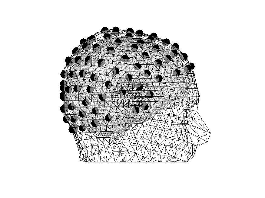
Figure 7: Electrodes are in meaningful places

Creating a source model (a volumetric grid (fit for beamformer and dipole analysis)) (Component 3)

The next step is to create a source model that indicates where our sources are. For beamformer and dipole analyses, so-called volumetric grids will do just fine. (For Minimum Norm Estimates, a source model, where sources are constrained to the cortical surface is needed, see for example this tutorial)

cfg             = [];
cfg.headmodel   = headmodel; % used to estimate extent of grid
cfg.resolution  = 0.01; % a source per 0.01 m -> 1 cm
cfg.inwardshift = 0.005; % moving sources 5 mm inwards from the skull, ...
                         % since BEM models may be unstable here

sourcemodel = ft_prepare_sourcemodel(cfg);

and plot it

figure
hold on
ft_plot_mesh(sourcemodel, 'vertexsize', 20);
ft_plot_headmodel(headmodel, 'facealpha', 0.5)
view(90, 0)

print -dpng sourcemodel.png

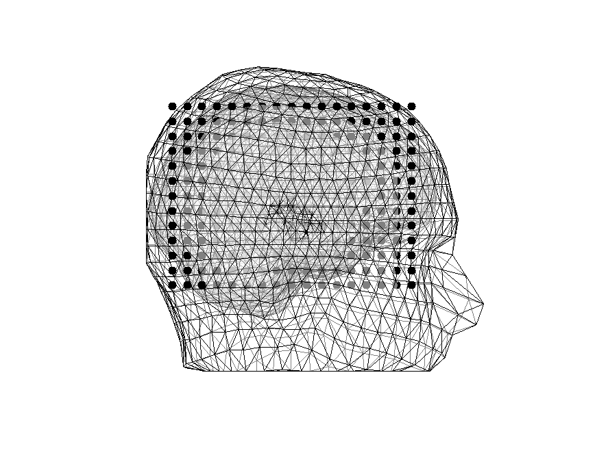
Figure 8: Head model overlain with source model (black dots)

and highlight the sources inside the brain (in red)

inside = sourcemodel;
outside = sourcemodel;

inside.pos = sourcemodel.pos(sourcemodel.inside, :);
outside.pos = sourcemodel.pos(~sourcemodel.inside, :);

figure
hold on
ft_plot_mesh(inside, 'vertexsize', 20, 'vertexcolor', 'red');
ft_plot_mesh(outside, 'vertexsize', 20)
ft_plot_headmodel(headmodel, 'facealpha', 0.1)
view(125, 10)

print -dpng sourcemodel_inside_outside.png

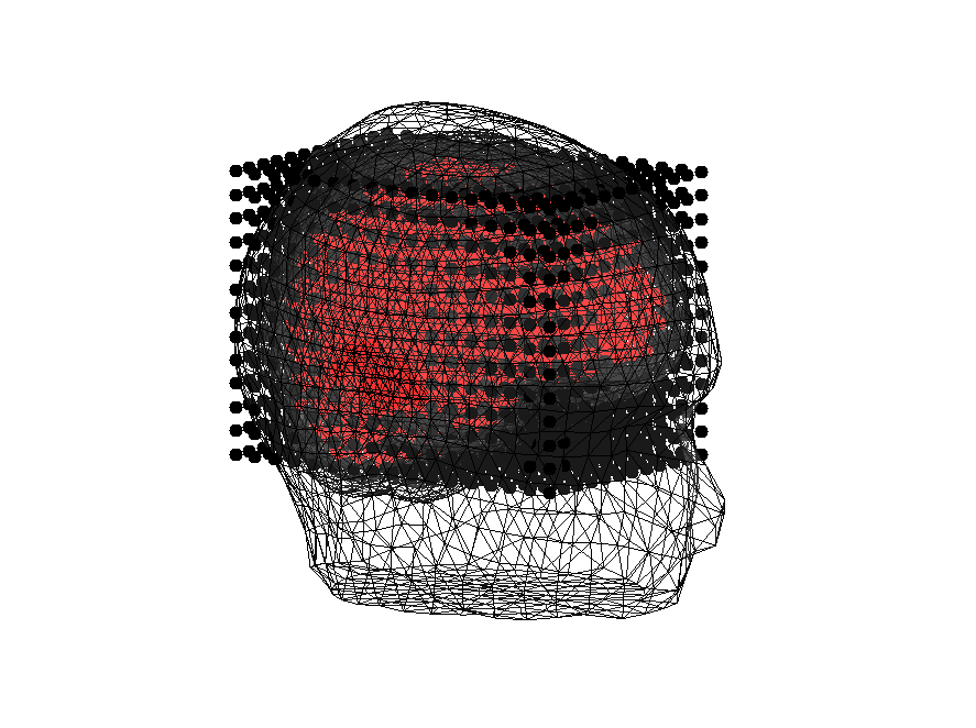
Figure 9: Head model overlain with sources outside (black dots) and sources inside the brain (red dots)

Estimating the lead field (Component 4)

cfg = [];
cfg.sourcemodel = sourcemodel;    %% where are the sources?
cfg.headmodel   = headmodel;      %% how do currents spread?
cfg.elec        = elec_realigned; %% where are the sensors?

% how do sources and sensors connect?
sourcemodel_and_leadfield = ft_prepare_leadfield(cfg);

Let’s have a look at the output of sourcemodel_and_leadfield

sourcemodel_and_leadfield =

                dim: [14 18 14]
                pos: [3528x3 double]
               unit: 'm'
             inside: [3528x1 logical]
                cfg: [1x1 struct]
          leadfield: {1x3528 cell}
              label: {128x1 cell}
    leadfielddimord: '{pos}_chan_ori'

• dim contains the dimensions of the grid in which the 3528 (14x18x14) sources are placed
• pos contains the xyz coordinates for the sources in the source model
• unit contains the unit of pos
• inside contains a logical vector indicating whether the source is a source or not
• cfg contains information about the call of ft_prepare_leadfield
• leadfield a cell array, where each cell (3528) contains a matrix of 128 rows (n channels) and 3 columns (_xyz-coordinates). (The ones that are outside the brain are empty though). For each channel-orientation pair, you get the electric potential measured given that the relevant source has an activation of 1 Am
• label contains the electrode names
• leadfielddimord indicates the dimension. Each cell is a position, which contains a matrix ordered by channels x orientations (xyz)

Plotting the lead field

It is always recommended to plot the lead fields alongside the electrodes and head model to see if things look okay. The code for this takes a bit more work as can be seen by the length of the code below. Note that we use a realistic source current of 100 nAm (sensory_dipole_current)

figure('units', 'normalized', 'outerposition', [0 0 0.5 0.5])
source_index = 1200; %% a superficial sources
sensory_dipole_current = 100e-9; % Am (realistic)

n_sensors = length(elec_realigned.label);

inside_sources = find(sourcemodel_and_leadfield.inside);
inside_index = inside_sources(source_index);
lead = sourcemodel_and_leadfield.leadfield{inside_index};
xs = zeros(1, n_sensors);
ys = zeros(1, n_sensors);
zs = zeros(1, n_sensors);
voltages = zeros(1, n_sensors);
titles = {'Lead field (x)' 'Lead field (y)' 'Lead field (z)'};

% get the xyz and norm

for sensor_index = 1:n_sensors
    this_x = lead(sensor_index, 1);
    this_y = lead(sensor_index, 2);
    this_z = lead(sensor_index, 3);
    this_norm = norm(lead(sensor_index, :));
    xs(sensor_index) = this_x * sensory_dipole_current;
    ys(sensor_index) = this_y * sensory_dipole_current;
    zs(sensor_index) = this_z * sensory_dipole_current;
    voltages(sensor_index) = this_norm * sensory_dipole_current;
end

% plot xyz
axes = {xs ys zs};

for axis_index = 1:3
    this_axis = axes{axis_index};
    subplot(1, 3, axis_index)
    hold on
    ft_plot_topo3d(elec_realigned.chanpos, this_axis, 'facealpha', 0.8)
    if strcmp(headmodel.type, 'dipoli')
        caxis([-10e-6, 10e-6])
    end
    c = colorbar('location', 'southoutside');
    c.Label.String = 'Lead field (V)';
    axis tight
    ft_plot_mesh(mesh_brain, 'facealpha', 0.10);
    ft_plot_sens(elec_realigned, 'elecsize', 20);
    title(titles{axis_index})
    plot3(sourcemodel_and_leadfield.pos(inside_index, 1), ...
      sourcemodel_and_leadfield.pos(inside_index, 2), ...
      sourcemodel_and_leadfield.pos(inside_index, 3), 'bo', ...
      'markersize', 20, 'markerfacecolor', 'r')
end

% plot norm

figure('units', 'normalized', 'outerposition', [0 0 0.5 0.85])
hold on
ft_plot_topo3d(elec_realigned.chanpos, voltages, 'facealpha', 0.8)
if strcmp(headmodel.type, 'dipoli')
    caxis([0, 10e-6])
end
c = colorbar('location', 'eastoutside');
c.Label.String = 'Lead field (V)';
axis tight
ft_plot_mesh(mesh_brain, 'facealpha', 0.10);
ft_plot_sens(elec_realigned, 'elecsize', 20);
title('Leadfield magnitude')
plot3(sourcemodel_and_leadfield.pos(inside_index, 1), ...
  sourcemodel_and_leadfield.pos(inside_index, 2), ...
  sourcemodel_and_leadfield.pos(inside_index, 3), 'bo', ...
  'markersize', 20, 'markerfacecolor', 'r')

view(-90, 0)

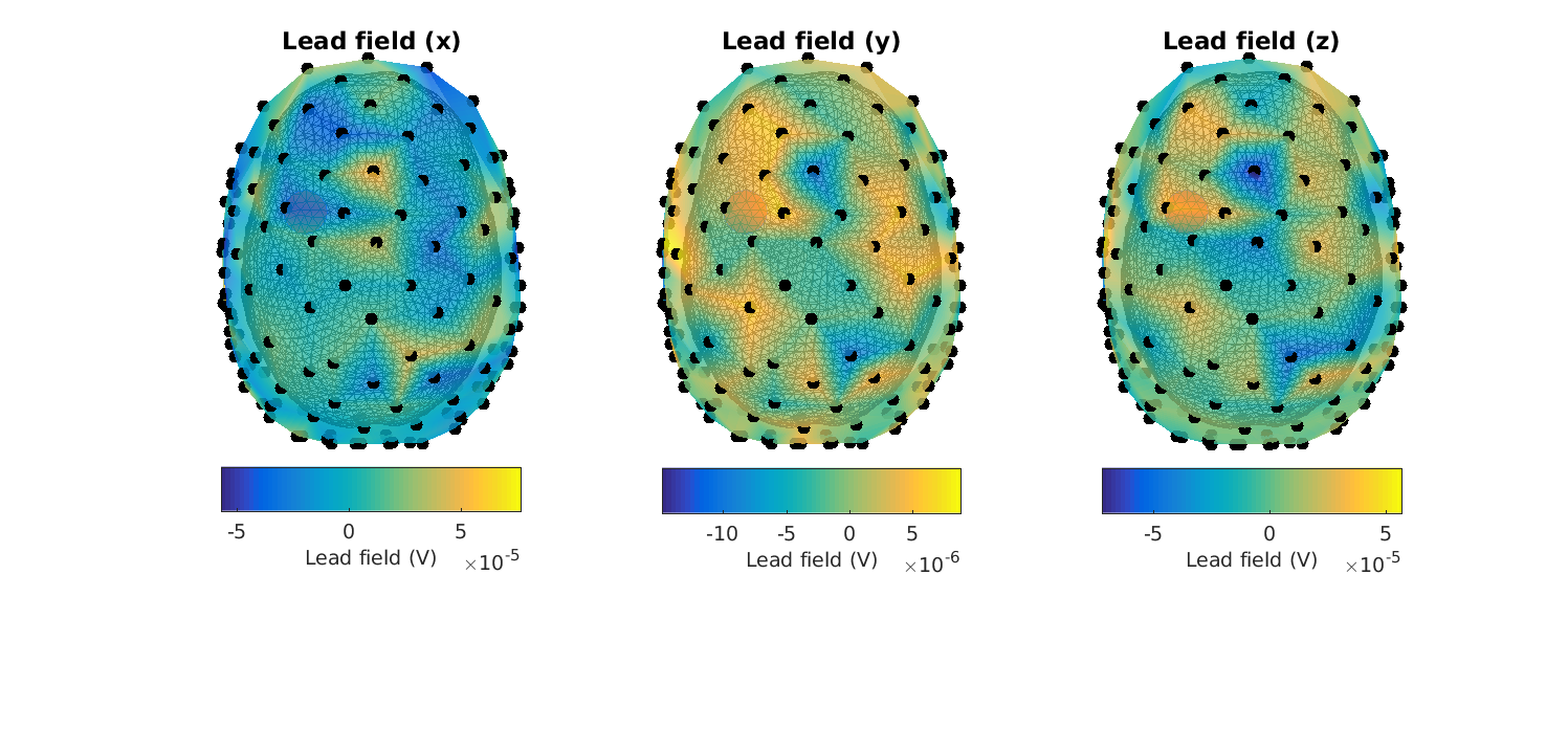
Figure 10: Lead fields in the XYZ-_directions for_ headmodel_bem for a superficial source. Note that there is something wrong.

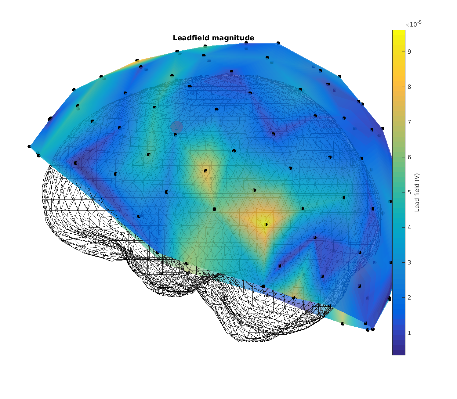
Figure 11: Magnitude of the lead fields for headmodel_bem for a superficial source. Note that there is something wrong.

Let’s change to the dipoli head model (load it if you cannot create it)

headmodel = headmodel_dipoli;

and run the code creating elec_realigned, sourcemodel and sourcemodel_and_leadfield again with headmodel as headmodel_dipoli

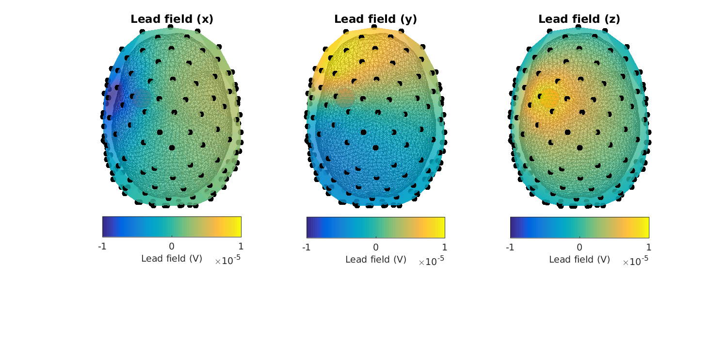
Figure 12: Lead fields in the XYZ-_directions for_ headmodel_dipoli for a superficial source

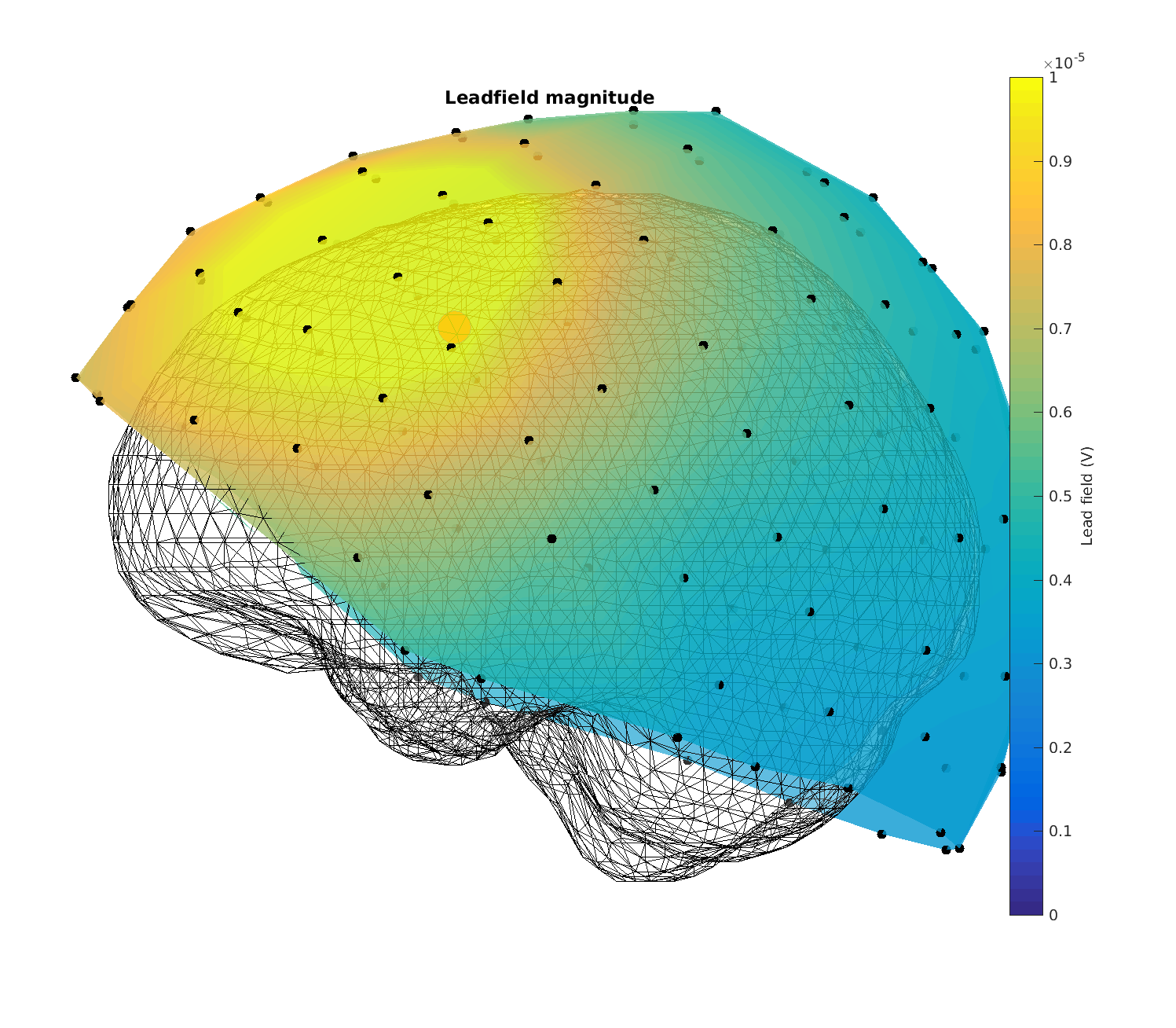
Figure 13: Magnitude of the lead fields for headmodel_dipoli for a superficial source

We can also plot the vectors - note that they are more or less normal to the scalp surface. Also note that we are using an unrealistic source current here, 1 mAm. This is just to make sure that they are visible. Do play around with it to see its effect.

% source_index 300 is central, 1200 is superficial

figure
hold on
ft_plot_sens(elec_realigned, 'elecsize', 40);
ft_plot_headmodel(headmodel, 'facealpha', 0.5);
view(90, 0)

source_index = 1200;
sensory_dipole_current = 1e-3; % Am (unrealistic)
n_sensors = length(elec_realigned.label);

inside_sources = find(sourcemodel_and_leadfield.inside);
inside_index = inside_sources(source_index);
lead = sourcemodel_and_leadfield.leadfield{inside_index};

for sensor_index = 1:n_sensors
    this_pos = elec_realigned.chanpos(sensor_index, :);
    this_lead = lead(sensor_index, :);
    this_voltage = this_lead * sensory_dipole_current;
    quiver3(this_pos(1), this_pos(2), this_pos(3), ...
            this_voltage(1), this_voltage(2), this_voltage(3), 'r', ...
            'linewidth', 3, 'markersize', 100);
end

plot3(sourcemodel_and_leadfield.pos(inside_index, 1), ...
      sourcemodel_and_leadfield.pos(inside_index, 2), ...
      sourcemodel_and_leadfield.pos(inside_index, 3), 'o', ...
      'markersize', 60, 'markerfacecolor', 'r')

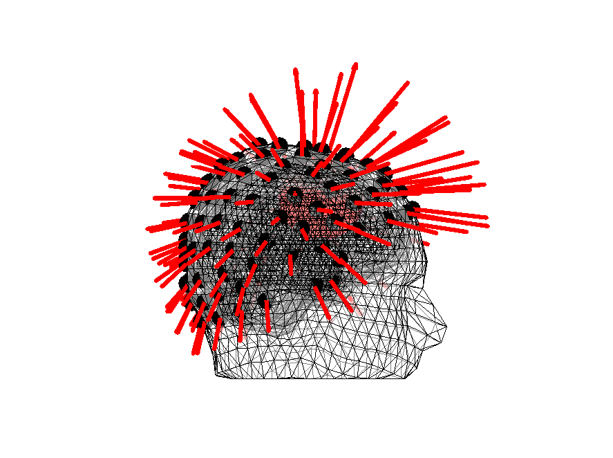
Figure 14: Orientations of the lead fields for headmodel_dipoli for a superficial source

Bonus: troubleshooting the meshes

The bemcp algorithm might have failed due to the meshes overlapping (brain, skull and scalp). One way to test this is to increase the number of vertices when creating the meshes at the expense of an increase in processing time. I tested it with a fine head model where all the meshes had 10,000 vertices. This also didn’t succeed. In other cases, you might succeed, so it might be worth trying. One reason that it might fail is that the segmented surfaces are “too” thin at places. The following code will exemplify this. First, we create a “binary” mri, where brain, skull and scalp are expressed binarily. Then a combined field is created.

mri_segmented_binary = mri_segmented; % make a copy

binary_brain = mri_segmented.brain;
binary_skull = mri_segmented.skull | mri_segmented.brain;
binary_scalp = mri_segmented.scalp | mri_segmented.skull | mri_segmented.brain;

mri_segmented_binary.combined = binary_scalp + binary_skull + binary_brain;

We subsequently plot this combined field at a location where the skin is very thin. Please have a look around and ascertain for yourself that these thin places exist

cfg              = [];
cfg.funparameter = 'combined';
cfg.location     = [-74 -4 30];

ft_sourceplot(cfg, mri_segmented_binary);

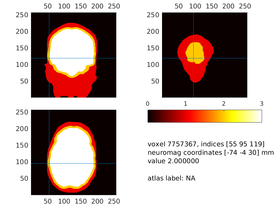
Figure 15: The brain (white), skull (yellow) and scalp surfaces (red). Notice how thin the scalp is at places, which will make the potentials (in the model) escape from the skull to the air around it directly

Which BEM algorithm to use?

If possible, you should use the OpenMEEG algorithm implemented in FieldTrip (in ft_prepare_headmodel use cfg.method = ‘openmeeg’. This may require some careful installation before it works, and it only works on Linux and Mac systems.

If you cannot make this work, then dipoli, which also only works on Linux and Mac systems (at the moment) is your next choice, and finally bemcp which works on all platforms.