Time-frequency analysis of EEG data

Introduction

In this tutorial, you can find information about the frequency and time-frequency analysis of a single subject’s EEG data. We will use both Fourier analysis with Hanning tapers and Morlet wavelets; and we will have a special focus on how to visualize the data. We will learn how to compare conditions in the frequency domain, looking at differences in beta band activity after left versus the right hand responses. You can familiarize yourself with the paradigm and data by reading the example dataset description.

Background

Oscillatory components contained in the ongoing EEG or MEG signal often show power changes relative to experimental events. These signals are not necessarily phase-locked to the event and will not be represented in event-related fields and potentials (Tallon-Baudry & Bertrand, 1999). The goal of this tutorial is to compute and visualize event-related changes by calculating time-frequency representations (TFRs) of power. This will be done using analyses based on Fourier analysis and wavelets.

Calculating time-frequency representations of power using Fourier analysis is done using a sliding time window. This time window can either have a fixed length independent of frequency, or the time window decreases in length with increased frequency. For each time window the power is calculated. Prior to calculating the power, a taper is multiplied with the data. The aim of the tapers is to reduce spectral leakage and control the frequency smoothing.

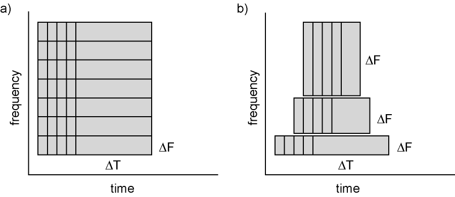
Figure: Time and frequency smoothing. (a) For a fixed length time window the time and frequency smoothing remains fixed. (b) For time windows that decrease with frequency, the temporal smoothing decreases and the frequency smoothing increases.

If you want to know more about tapers/window functions you can have a look at this Wikipedia site. Note that Hann window is another name for the Hanning window used in this tutorial.

Procedure

To calculate the time-frequency representation for the example dataset we will perform the following steps:

• Read the data into Matlab using ft_definetrial and ft_preprocessing
• Compute the power values for each frequency bin and each time bin using the function ft_freqanalysis
• Visualize the results. This can be done by creating time-frequency plots for one (ft_singleplotTFR) or several channels (ft_multiplotTFR), or by creating a topographic plot for a specified time- and frequency interval (ft_topoplotTFR).

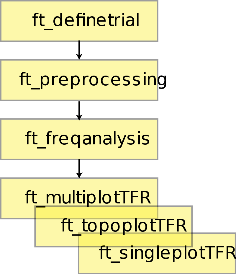
Figure: Schematic overview of the steps in time-frequency analysis

Preprocessing EEG data

The first step is to read the data using the function ft_preprocessing. With the aim to reduce boundary effects occurring at the start and the end of the trials, it is recommended to read larger time intervals than the time period of interest. In this example, the time of interest is from -1.0 s to 1.5 s (t = 0 s defines the time of response); however, the script reads the data from -1.5 s to 2.0 s.

The EEG dataset that we use in this tutorial is available as BrainVision EEG files from our download server. You should download the binary data file, the header file, and the text marker file. You can find out more about the BrainVision file format in this overview.

We will focus on two conditions from this dataset: whether the participant responded with the left or the right index finger.

Read and epoch data

cfg = [];
cfg.dataset = 'oddball1_mc_downsampled_eeg.vhdr';

% define trials based on responses
cfg.trialdef.prestim    = 1.5;
cfg.trialdef.poststim   = 2.0;
cfg.trialdef.eventtype  = 'STI102';  % name of trigger channel
cfg.trialdef.eventvalue = [256, 4096];  % 256: button press left;
                                        % 4096: button press right
cfg.trialfun            = 'ft_trialfun_general';
cfg                     = ft_definetrial(cfg);

% preprocess EEG data
cfg.demean              = 'yes';
cfg.dftfilter           = 'yes';
cfg.dftfreq             = [50 100];
cfg.reref               = 'yes';  % re-referencing
cfg.refchannel          = 'all';

data                    = ft_preprocessing(cfg);

Computing power spectra

At first, we will look at the frequency content in the data using a Fourier transform using a Fourier transform with a Hanning window by using ft_freqanalysis. This is not time resolved, but gives us a power estimate per frequency over the whole time window. We calculate this separately for the trials where the participant responded with the left and the right index finger. We will calculate and visualize the power for a selected central EEG channel.

cfg         = [];
cfg.output  = 'pow';
cfg.channel = 'EEG126';
cfg.method  = 'mtmfft';
cfg.taper   = 'hanning';
cfg.foi     = 7:40;

cfg.trials   = find(data.trialinfo(:,1) == 256);
spectr_left  = ft_freqanalysis(cfg, data);

cfg.trials   = find(data.trialinfo(:,1) == 4096);
spectr_right = ft_freqanalysis(cfg, data);

The output of ft_freqanalysis is a structure with the following elements:

spectr_left =
    label: {'EEG126'}      % Channel names
   dimord: 'chan_freq'     % Dimensions contained in powspctrm, channels x frequencies
     freq: [1x34 double]   % Array of frequencies of interest (the elements of freq may be different from your cfg.foi input depending on your trial length)
powspctrm: [1x34 double]   % Array containing the power values
      cfg: [1x1 struct]    % Settings used in computing this frequency decomposition

The field spectr_left.powspctrm contains the power values for each specified frequency in the left response condition.

Visualizing the power spectra

We can visualize the power spectra from both conditions in one plot using MATLAB’s plotting function.

figure;
hold on;
plot(spectr_left.freq, (spectr_left.powspctrm), 'linewidth', 2)
plot(spectr_left.freq, (spectr_right.powspctrm), 'linewidth', 2)
legend('Button press left', 'Button press right')
xlabel('Frequency (Hz)')
ylabel('Power (\mu V^2)')

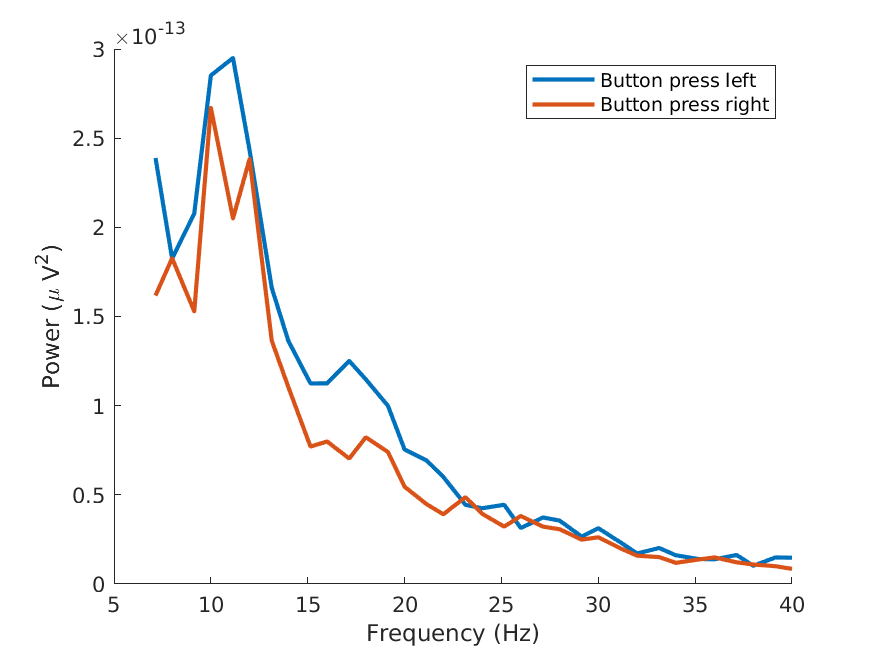
Figure: Power spectra for both conditions in a right central electrode.

Time-frequency analysis with a Hanning taper and fixed window length

Here, we will look at calculating time-frequency representations using Hanning tapers. When choosing a fixed window length for the sliding window, the frequency resolution is defined according to the length of this time window (compare delta T in the first figure of this tutorial). The frequency resolution (delta F in the first figure) equals 1/delta T (the length of time window in sec). Thus, a 500 ms time window as we choose here results in a 2 Hz frequency resolution (1/0.5 sec= 2 Hz). This means that power can be calculated for 2 Hz, 4 Hz, 6 Hz etc., as an integer number of cycles must fit in the time window.

Since we have two conditions (responses with left and right index finger), we will calculate the output separately for both conditions so that we can compare them. We select the trials based on the .trialinfo field and the trigger values for left hand (256) and right hand responses (4096).

cfg            = [];
cfg.output     = 'pow';
cfg.channel    = 'all';
cfg.method     = 'mtmconvol';
cfg.taper      = 'hanning';
cfg.toi        = -1 : 0.10 : 1.5;
cfg.foi        = 2:2:40;
cfg.t_ftimwin  = ones(size(cfg.foi)) * 0.5;

cfg.trials     = find(data.trialinfo(:,1) == 256);
tfr_left       = ft_freqanalysis(cfg, data);

cfg.trials     = find(data.trialinfo(:,1) == 4096);
tfr_right      = ft_freqanalysis(cfg, data);

If we compare the output of ft_freqanalysis to what we obtained when computing the power spectra (see above), we can see that the data now also contains a time dimension:

tfr_left =
    label: {128x1 cell}
   dimord: 'chan_freq_time'
     freq: [2 4 6 8 10 12 14 16 18 20 22 24 26 28 30 32 34 36 38 40]
     time: [1x26 double]
powspctrm: [128x20x26 double]
      cfg: [1x1 struct]

Note especially how the output now contains a field time and that powspctrm is 3-dimensional. The dimension order field dimord tells us that time is the third dimension of the power output matrix powspctrm.

Visualization

To visualize the event-related power changes, a normalization with respect to a baseline interval will be performed. There are two possibilities for normalizing:

• Subtracting, for each frequency, the average power in a baseline interval from all other power values. This gives, for each frequency, the absolute change in power with respect to the baseline interval.
• Expressing the raw power values as the relative increase or decrease with respect to the power in the baseline interval (for each frequency): active period divided by baseline. Note that the relative baseline is expressed as a ratio; i.e., no change is represented by 1.

Let’s first look at the topographical representation of the power changes in a specified time-interval using ft_topoplotTFR. We choose to look at 400 to 800 ms and plot the data with an absolute baseline.

cfg              = [];
cfg.baseline     = [-0.5 -0.1];
cfg.baselinetype = 'absolute';
cfg.xlim         = [0.4 0.8];  % specified in seconds
cfg.ylim         = [16 24];    % we only plot the beta band
cfg.zlim         = 'maxabs';
cfg.marker       = 'on';
cfg.colorbar     = 'yes';
cfg.layout       = 'natmeg_customized_eeg1005.lay';

figure;
ft_topoplotTFR(cfg, tfr_left);
title('Left hand reaction');

figure;
ft_topoplotTFR(cfg, tfr_right);
title('Right hand reaction');

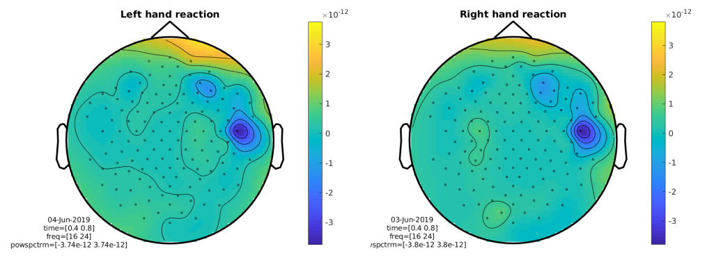
Figure: Topographic representation of absolute power changes to baseline.

Using a relative baseline

Let’s take a look at what happens when instead of an absolute baseline we use a relative baseline:

cfg              = [];
cfg.baseline     = [-0.5 -0.1];
cfg.baselinetype = 'relative';  % we use a relative baseline
cfg.xlim         = [0.4 0.8];
cfg.ylim         = [16 24];
cfg.zlim         = 'maxabs';
cfg.marker       = 'on';
cfg.colorbar     = 'yes';
cfg.layout       = 'natmeg_customized_eeg1005.lay';

figure;
ft_topoplotTFR(cfg, tfr_left);
title('Left hand reaction');

figure;
ft_topoplotTFR(cfg, tfr_right);
title('Right hand reaction');

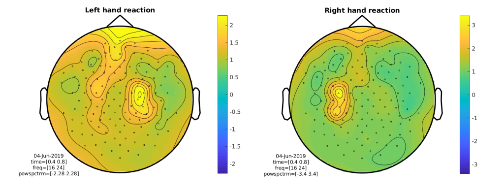
Figure: Topographic representation of relative power changes to baseline.

This looks better! We can also plot the time-resolved activity using ft_singleplotTFR. Let’s choose the same central electrode as we used above for the power spectra:

cfg          = [];
cfg.colorbar = 'yes';
cfg.zlim     = 'maxabs';
cfg.ylim     = [10 Inf];  % plot alpha band upwards
cfg.layout   = 'natmeg_customized_eeg1005.lay';
cfg.channel  = 'EEG126';

figure;
ft_singleplotTFR(cfg, tfr_left);
title('Left hand reaction');

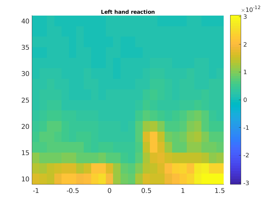
Figure: Time-frequency representation of power at a central electrode.

Plot the difference between conditions

We now want to collapse the information of both conditions by comparing them. One possibility is to take the difference between the conditions: we subtract the two power spectra and then divide them by their sum - this normalizes the difference by the common activity. This can conveniently be done using ft_math:

cfg = [];
cfg.parameter    = 'powspctrm';
cfg.operation    = '(x1-x2)/(x1+x2)';

tfr_difference = ft_math(cfg, tfr_right, tfr_left);

cfg = [];
cfg.xlim         = [0.4 0.8];
cfg.ylim         = [16 24];
cfg.zlim         = 'maxabs';
cfg.marker       = 'on';
cfg.colorbar     = 'yes';
cfg.layout       = 'natmeg_customized_eeg1005.lay';

figure;
ft_topoplotTFR(cfg, tfr_difference);
title('Left vs right hand reaction');

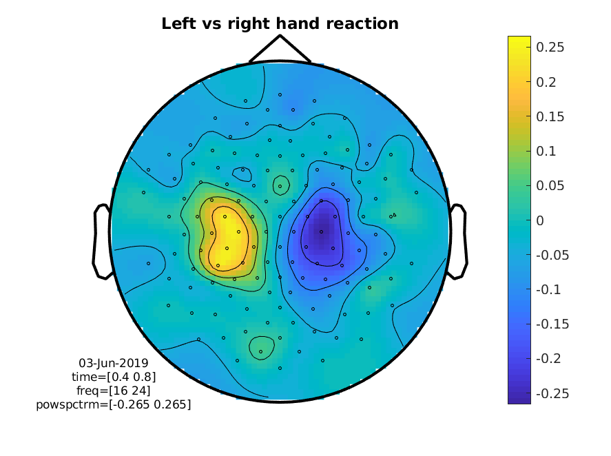
Figure: Topographic representation of the time-frequency representations of the difference in beta power, between left and right response.

Bonus: Recreate the analysis using Morlet wavelets

An alternative for calculating TFRs is to use wavelets instead of Fourier analysis. A special thing about wavelets is that their temporal resolution scales with frequency (for a given number of cycles). In our analysis above, we used a sliding time window that was fixed, i.e., it was (in our case) always 500 ms long, irrespective of the frequency. This means that for higher frequencies, more cycles fit into this window: for example, 5 cycles of a 10 Hz oscillation fit in 500 ms, whereas for 30 Hz we can fit 15 cycles. For wavelets, we instead specify the number of cycles (equal to the width of the wavelet) directly, setting the parameter cfg.width.

Let’s calculate the time-frequency representation of our data using Morlet wavelets (i.e., using wavelets that were created using a Gaussian taper):

cfg            = [];
cfg.output     = 'pow';
cfg.channel    = 'all';
cfg.method     = 'wavelet';
cfg.width      = 7;
cfg.toi        = -1 : 0.05 : 1.5;
cfg.foi        = 1:40;

cfg.trials     = find(data.trialinfo(:,1) == 256);
wave_left      = ft_freqanalysis(cfg, data);

cfg.trials     = find(data.trialinfo(:,1) == 4096);
wave_right     = ft_freqanalysis(cfg, data);

Plot the difference between conditions

As for our first analysis, we want to look at the difference between the conditions, so we use ft_math again. We then visualize the results looking at the same channels as above.

cfg            = [];
cfg.parameter  = 'powspctrm';
cfg.operation  = '(x1-x2)/(x1+x2)';

wave_difference = ft_math(cfg, wave_right, wave_left);

cfg          = [];
cfg.colorbar = 'yes';
cfg.zlim     = 'maxabs';
cfg.layout   = 'natmeg_customized_eeg1005.lay';
cfg.channel  = 'EEG126';

figure;
ft_singleplotTFR(cfg, wave_difference);
title('Left vs right hand reaction');

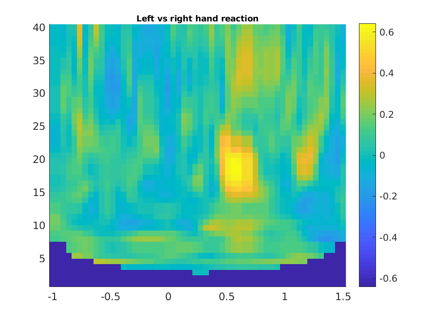
Figure: Time-frequency representations of power calculated using Morlet wavelets, difference between the conditions.