workshop / practicalmeeg2022 / handson_sensoranalysis /
Time-frequency analysis using Hanning window, multitapers and wavelets
This tutorial was written specifically for the PracticalMEEG workshop in Aix-en-Provence in December 2022 and is part of a coherent sequence of tutorials. It is an adjusted version of the time-frequency analysis tutorial and an updated version of the corresponding tutorial for Paris 2019.
Introduction
In this tutorial you can find information about the time-frequency analysis of a single subject’s MEG data using a Hanning window, multitapers and wavelets. This tutorial also shows how to visualize the results.
Here, we will work on the face recognition dataset. This tutorial is a continuation from the raw2erp tutorial.
Background
Oscillatory components contained in the ongoing EEG or MEG signal often show power changes relative to experimental events. These signals are not necessarily phase-locked to the event and will not be represented in event-related fields and potentials (Tallon-Baudry and Bertrand (1999)). The goal of this section is to compute and visualize event-related changes by calculating time-frequency representations (TFRs) of power. This will be done using analysis based on Fourier analysis and wavelets. The Fourier analysis will include the application of multitapers (Mitra and Pesaran (1999), Percival and Walden (1993)) which allow a better control of time and frequency smoothing.
Calculating time-frequency representations of power is done using a sliding time window. This can be done according to two principles: either the time window has a fixed length independent of frequency, or the time window decreases in length with increased frequency. For each time window the power is calculated. Prior to calculating the power one or more tapers are multiplied with the data. The aim of the tapers is to reduce spectral leakage and control the frequency smoothing.
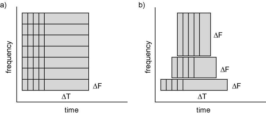
Figure: Time and frequency smoothing. (a) For a fixed length time window the time and frequency smoothing remains fixed. (b) For time windows that decrease with frequency, the temporal smoothing decreases and the frequency smoothing increases.
If you want to know more about tapers/ window functions you can have a look at this Wikipedia site. Note that Hann window is another name for Hanning window used in this tutorial. There is also a Wikipedia site about multitapers, to take a look at it click here.
Procedure
To calculate the time-frequency analysis for the example dataset we will perform the following steps:
- Read the data into MATLAB using the same strategy as in the raw2erp tutorial.
- Compute the power values for each frequency bin and each time bin using the function ft_freqanalysis
- Visualize the results. This can be done by creating time-frequency plots for one with ft_singleplotTFR or several channels with ft_multiplotTFR, or by creating a topographic plot for a specified time- and frequency interval with ft_topoplotTFR.
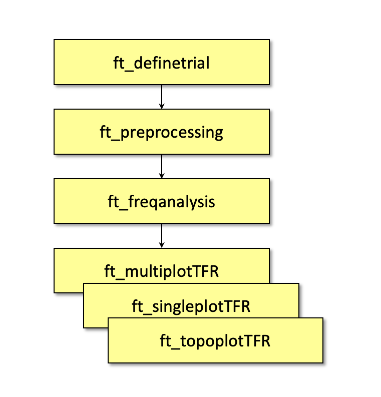
Figure: Schematic overview of the steps in time-frequency analysis
This tutorial shows four types of time-frequency analysis. You can find each of them in the table of content under the titles: Time-frequency analysis I, II, III and IV. If you are interested in a detailed description about how to visualize the results, look at the Visualization section.
The first step is to read the data using the function ft_preprocessing. To reduce boundary effects at the start and the end of the trials, it is recommended to read slightly larger time intervals than the time period of interest. In this example, the time of interest is from -0.6 s to 1.3 s, where t=0 defines the time of stimulus); however, for reasons that will become clear later, the script reads the data from -0.8 s to 1.5 s.
Preprocessing the data
The ft_freqanalysis function requires a ‘raw’ data structure, which is the output of ft_preprocessing. In the following code section, we duplicate the preprocessing part of the raw2erp tutorial tutorial, with a few important modifications. As mentioned above, the epoch length is increased to account for boundary effects. Moreover, we will not apply a bandpass filter to the data (why not?) and will only read in the MEG data. The execution of the following chunk of code takes some time. The precomputed data are in the derivatives/sensoranalysis/sub-01 folder, and can also be loaded from there:
subj = datainfo_subject(1);

subj.trl = cell(6,1);
for run_nr = 1:6

  cfg = [];
  cfg.dataset = subj.megfile{run_nr};
  cfg.readbids = 'no'; % it looks like BIDS, but is not complete

  % this is what we can see in the BIDS events.tsv file
  Famous      = [5 6 7];
  Unfamiliar  = [13 14 15];
  Scrambled   = [17 18 19];

  cfg.trialfun = 'ft_trialfun_general';
  cfg.trialdef.eventtype = 'STI101';
  cfg.trialdef.eventvalue = [Famous Unfamiliar Scrambled];
  cfg.trialdef.prestim = 0.5;
  cfg.trialdef.poststim = 1.2;

  cfg = ft_definetrial(cfg);

  % remember the trial definition for each run
  subj.trl{run_nr} = cfg.trl;

end % for each run

rundata = cell(1,6);
for run_nr = 1:6

  cfg         = [];
  cfg.dataset = subj.megfile{run_nr};
  cfg.trl     = subj.trl{run_nr};

  % MEG specific settings, minimal preprocessing
  cfg.channel = 'MEG';
  cfg.demean  = 'yes';
  cfg.coilaccuracy = 0;
  data_meg    = ft_preprocessing(cfg);

  cfg            = [];
  cfg.resamplefs = 300;
  data_meg       = ft_resampledata(cfg, data_meg);

  % remember the data from this run
  rundata{run_nr} = data_meg;
end % for each run

data = ft_appenddata([], rundata{:});
clear rundata;
Alternatively, you can also use the sub-01_data.mat data file that is shared on our download server.
filename = fullfile(subj.outputpath, 'sensoranalysis', subj.name, sprintf('%s_data.mat', subj.name));
% save(filename, 'data');
load(filename, 'data');
Frequency analysis (not time-resolved)
Before we go to time-frequency analysis, let’s first look at how the power spectrum of the signal looks like without considering the stimulus that is presented at t=0.
We can compute the power using the mtmfft method using a single hanning window.
cfg = [];
cfg.method = 'mtmfft';
cfg.taper = 'hanning';
freq = ft_freqanalysis(cfg, data);
To plot the data, we can use ft_singleplotER and ft_multiplotER. Note that the same functions are used for ERPs and non-time-resolved spectra, both types of data are represented in a 2D matrix, which is channels-by-time or channels-by-frequency. Rather than plotting time along the horizontal axis, for the power spectrum the functions will plot the frequency along the horizontal axis.
However, we can also use plain MATLAB plotting functions. Let’s look at a specific MEG channel
% this shows that MEG0741 corresponds to channel 84
find(strcmp(freq.label, 'MEG0741'))

figure
plot(freq.freq, freq.powspctrm(84,:));
xlabel('frequency')
ylabel('power')
Rather than plotting power along a linear axis, we can also use a logarithmic axis.
figure
semilogy(freq.freq, freq.powspctrm(84,:))
xlabel('frequency')
ylabel('power')
Or we can log transform the data ourselves. The following converts the data into decibel (dB).
figure
plot(freq.freq, 10*log10(freq.powspctrm(84,:)));
xlabel('frequency')
ylabel('power (dB)')
grid on
set(gca, 'XTick', 0:10:150)
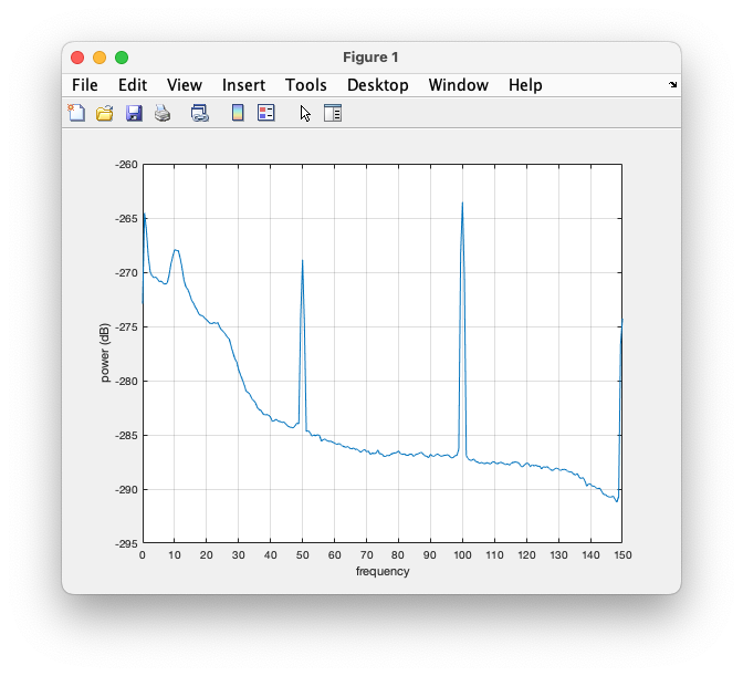
Figure: Power spectrum for channel MEG0741
We can see that the power spectrum ranges from 0 to 150 Hz, which is due to the data being downsampled from 1100 to 300 Hz and the Nyquist frequency is 1/2 times the sampling rate. We can also see the effect of the anti-aliasing filter around 140 Hz, which was applied prior to downsampling.
Furthermore, we see clear peaks at 50, 100 and 150 Hz, corresponding to the line-noise and its harmonics. There is quite some low-frequency noise below 5 Hz (which would probably be way less if we would have worked with the artifact-cleaned data). There is an alpha peak around 10 Hz, and not really a peak but rather a “shoulder” at 25 Hz, corresponding to the beta band.
If we would want to continue all subsequent analysis with the power converted to decibel, we could use the ft_math function to convert the powspctrm field to dB. That function can also be used to do mathematical operations on data structures, such as computing the difference between ERPs or computing the ratio between powerspectra. The following implements the dB transformation:
cfg = [];
cfg.operation = '10*log10(x1)';
cfg.parameter = 'powspctrm'; % this is represented by x, and x1 refers to the first (and only) input data structure
freq_db = ft_math(cfg, freq);
Since the power spectrum averaged over all trials shows a nice alpha peak, we could also check whether the alpha power increases over time. That is similar to how we computed the ERP image: we recompute the power spectrum, now only for one channel (to speed it up and use less memory) and we plot a color coded version of the trials-by-frequencies matrix.
cfg = [];
cfg.method = 'mtmfft';
cfg.taper = 'hanning';
cfg.keeptrials = 'yes';
cfg.channel = 'MEG0741';
freq_MEG0741 = ft_freqanalysis(cfg, data);

imagesc(10*log10(squeeze(freq_MEG0741.powspctrm)))
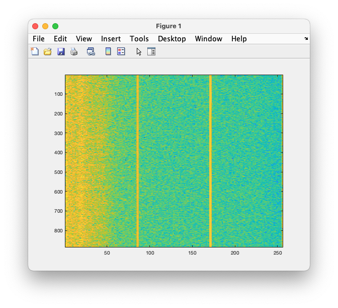
Figure: Power spectrum for channel MEG0741 over the whole course in the experiment
There is a FAQ that shows how to use a similar strategy to do time-frequency analysis on continuous data.
Time-frequency analysis I
Hanning taper, fixed window length
Here, we will describe how to calculate time frequency representations using Hanning tapers. When choosing for a fixed window length procedure, the frequency resolution is defined according to the length of the time window (delta T). The frequency resolution (delta f in figure 1) = 1/length of time window in sec (delta T in figure 1). Thus, a 400 ms time window results in a 2.5 Hz frequency resolution (1/0.4 sec= 2.5 Hz) meaning that power can be calculated for frequency bins centered at 2.5 Hz, 5 Hz, 7.5 Hz etc. An integer number of cycles must fit in the time window.
After reading and preprocessing the data, we can compute the time-frequency representation, which we do here for each of the conditions separately:
cfg        = [];
cfg.method = 'mtmconvol';
cfg.output = 'pow';
cfg.foi    = 2.5:2.5:30;
cfg.t_ftimwin = ones(1,numel(cfg.foi)).*0.4;
cfg.taper  = 'hanning';
cfg.toi    = (-0.8:0.05:1.3);
cfg.pad    = 4;

cfg.trials = ismember(data.trialinfo(:,1), Famous);
freqlow_famous = ft_freqanalysis(cfg, data);

cfg.trials = ismember(data.trialinfo(:,1), Unfamiliar);
freqlow_unfamiliar = ft_freqanalysis(cfg, data);

cfg.trials = ismember(data.trialinfo(:,1), Scrambled);
freqlow_scrambled = ft_freqanalysis(cfg, data);
Regardless of the method used for calculating the TFR, the output format is identical. It is a structure with the following fields:
freqlow_famous =

struct with fields:

    label: {306x1 cell}
   dimord: 'chan_freq_time'
     freq: [2.5000 5 7.5000 10 12.5000 15 17.5000 20 22.5000 25 27.5000 30]
     time: [1x43 double]
powspctrm: [306x12x43 double]
     elec: [1x1 struct]
     grad: [1x1 struct]
      cfg: [1x1 struct]
The ‘powspctrm’ field contains the temporal evolution of the raw power values for each specified channel and frequency bin. The ‘freq’ and ‘time’ fields represent the center points of each frequency and time bin in Hz and s. Note that each power value is not a ‘point estimate’, but always has some temporal and spectral extent.
Visualization
This part of the tutorial shows how to visualize the results of any type of time-frequency analysis.
To visualize the event-related power changes, a normalization with respect to a baseline interval will be performed. There are two possibilities for normalizing:
- Subtracting, for each frequency, the average power in a baseline interval from all other power values. This gives, for each frequency, the absolute change in power with respect to the baseline interval.
- Expressing, for each frequency, the raw power values as the relative increase or decrease with respect to the power in the baseline interval. This means active period/baseline. Note that the relative baseline is expressed as a ratio; i.e. no change is represented by 1.
There are three ways of graphically representing the data: 1) time-frequency plots of all channels, in a quasi-topographical layout, 2) time-frequency plot of an individual channel (or average of several channels), 3) topographical 2-D map of the power changes in a specified time and frequency window.
The function ft_multiplotTFR plots the TFRs from all the magnetometer sensors. Settings can be adjusted in the cfg structure, for example:
cfg = [];
cfg.baseline     = [-0.6 -0.2];
cfg.baselinetype = 'absolute';
cfg.zlim         = [-5e-27 5e-27];
cfg.showlabels   = 'yes';
cfg.layout       = 'neuromag306mag_helmet.mat';
figure; ft_multiplotTFR(cfg, freqlow_famous);
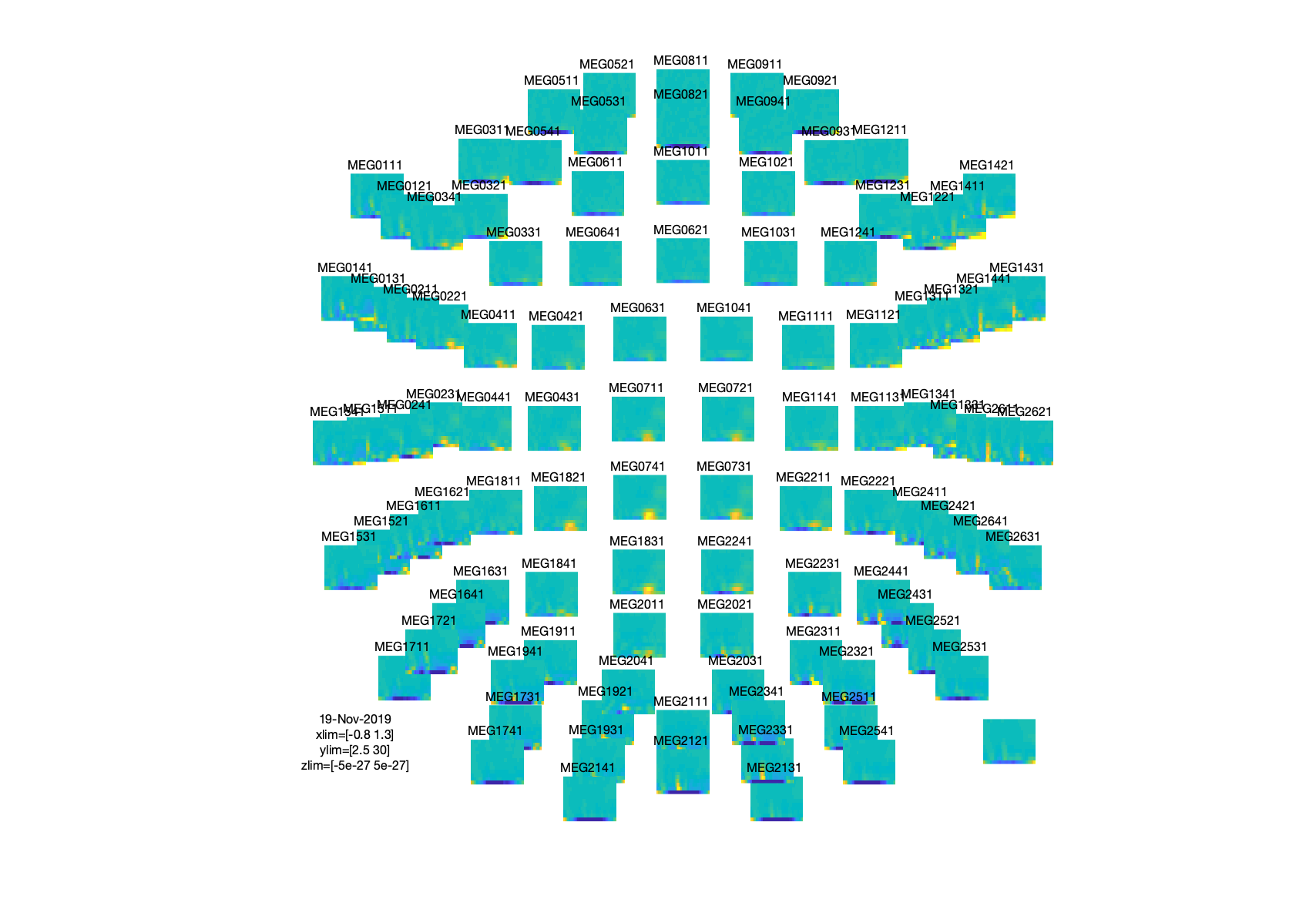
Figure: Time-frequency representations calculated using ft_freqanalysis. Plotting was done with ft_multiplotTFR)
The options cfg.baseline and cfg.baselinetype results in baseline correction of the data. Baseline correction can also be applied directly by calling ft_freqbaseline. Moreover, you can combine the various visualization options/functions interactively to explore your data. Currently, this is the default plotting behavior because the configuration option cfg.interactive='yes' is activated unless you explicitly select cfg.interactive='no' before calling ft_multiplotTFR to deactivate it. See also the plotting tutorial for more details.
An interesting effect seems to be present in the TFR of sensor MEG0731. To make a plot of a single channel you can make a selection with your mouse in the multiplot and click on it, or you can use ft_singleplotTFR.
cfg = [];
cfg.baseline     = [-0.6 -0.2];
cfg.baselinetype = 'absolute';
cfg.maskstyle    = 'saturation';
cfg.zlim         = [-5e-27 5e-27];
cfg.channel      = 'MEG0731';
figure; ft_singleplotTFR(cfg, freqlow_famous);
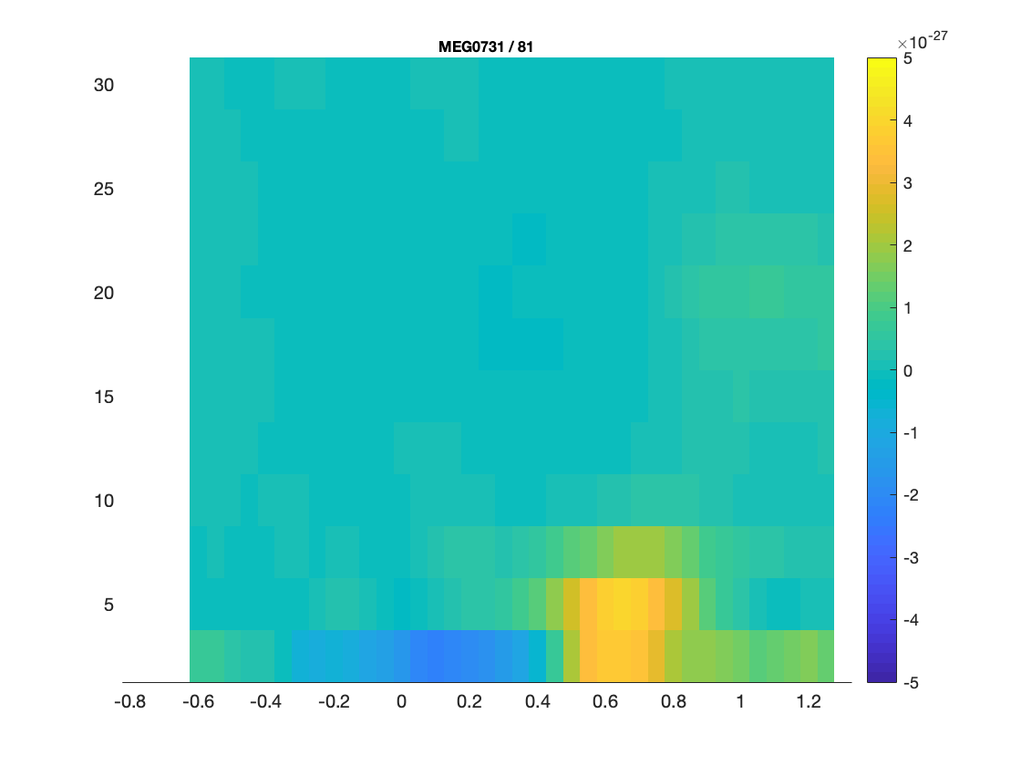
Figure: The time-frequency representation of a single sensor obtained using ft_singleplotTFR
If you see artifacts in your figure, see this FAQ.
From the previous figure you can see that there is an increase in power around 5 Hz in the time interval 0.6 to 0.8 s after stimulus onset. To show the topography of this ‘theta’ power increase you can use the function ft_topoplotTFR.
cfg = [];
cfg.layout       = 'neuromag306mag_helmet.mat'
cfg.baseline     = [-0.6 -0.2];
cfg.baselinetype = 'absolute';
cfg.xlim         = [0.6 0.8];
cfg.zlim         = [-5e-27 5e-27];
cfg.ylim         = [15 20];
cfg.marker       = 'on';
figure; ft_topoplotTFR(cfg, freqlow_famous);
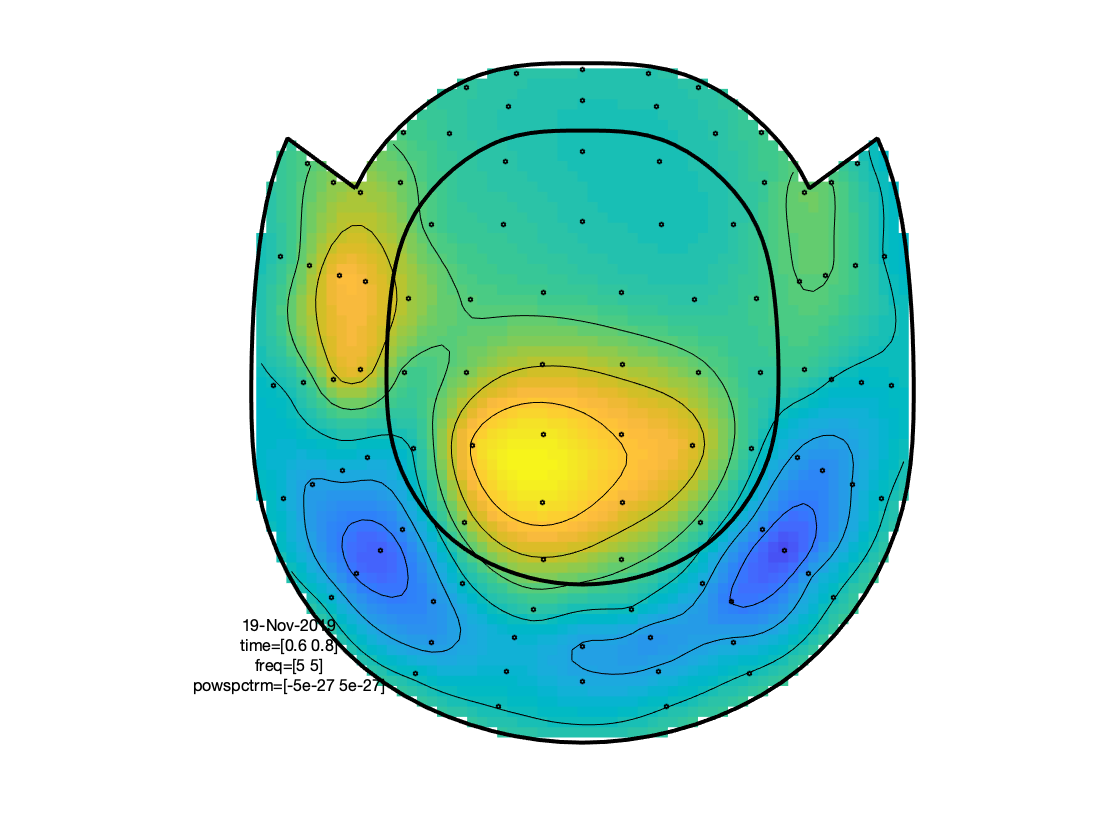
Figure: A topographic representation of the time-frequency representations (15 - 20 Hz, 0.9 - 1.3 s post stimulus) obtained using ft_topoplotTFR
Exercise 1
Plot the power with respect to a relative baseline (hint: use cfg.zlim=[0 2.0] and use the cfg.baselinetype option)
How are the responses different? Discuss the assumptions behind choosing a relative or absolute baseline.
Exercise 2
Plot the TFR of sensor MEG1921. How do you account for the increased power at ~100-200 ms? Hint: compare it to the ERFs.
Exercise 3
Visualize the TFR of the gradiometers. Use what you have learnt from the raw2erp tutorial to first combine the horizontal and planar gradient channels into a single estimate.
Time-frequency analysis II
Hanning taper, frequency dependent window length
It is also possible to calculate the TFRs with respect to a time window that varies with frequency. Typically the time window gets shorter with an increase in frequency. The main advantage of this approach is that the temporal smoothing decreases with higher frequencies, leading to increased sensitivity to short-lived effects. However, an increased temporal resolution is at the expense of frequency resolution (why?). We will here show how to perform a frequency-dependent time-window analysis, using a sliding window Hanning taper based approach. The approach is very similar to wavelet analysis. A wavelet analysis performed with a Morlet wavelet mainly differs by applying a Gaussian shaped taper.
The analysis is best done by first selecting the numbers of cycles per time window which will be the same for all frequencies. For instance if the number of cycles per window is 7, the time window is 1000 ms for 7 Hz (1/7 x 7 cycles); 700 ms for 10 Hz (1/10 x 7 cycles) and 350 ms for 20 Hz (1/20 x 7 cycles). The frequency can be chosen arbitrarily - however; too fine a frequency resolution is just going to increase the redundancy rather than providing new information.
Below is the configuration for a 7-cycle time window. The calculation is only done for one sensor (MEG0741) but it can of course be extended to all sensors.
cfg              = [];
cfg.output       = 'pow';
cfg.channel      = 'MEG0741';
cfg.method       = 'mtmconvol';
cfg.taper        = 'hanning';
cfg.foi          = 2:1:30;
cfg.t_ftimwin    = 7./cfg.foi;  % 7 cycles per time window
cfg.toi          = -0.8:0.05:1.5;
cfg.trials       = find(data.trialinfo(:,1)==1);
TFRhann7         = ft_freqanalysis(cfg, data);
To plot the result use ft_singleplotTFR:
cfg              = [];
cfg.baseline     = [-0.5 -0.1];
cfg.baselinetype = 'relchange';
cfg.maskstyle    = 'saturation';
cfg.zlim         = [-1 1];
cfg.channel      = 'MEG0741';
cfg.interactive  = 'no';
figure; ft_singleplotTFR(cfg, TFRhann7);
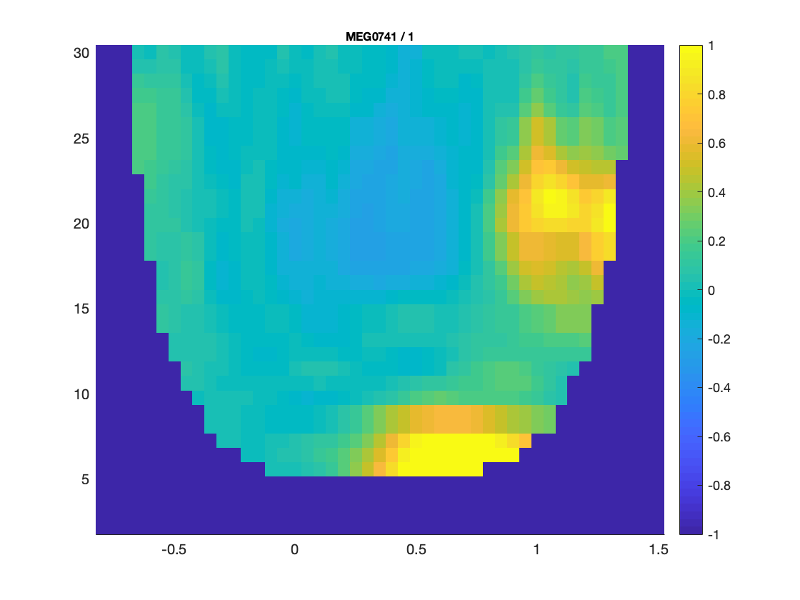
Figure: A time-frequency representation of channel MEG0741 obtained using ft_singleplotTFR
If you see artifacts in your figure, see this FAQ.
Note the boundary effects, in particular for the lower frequency bins, i.e. the blue (or white) region in the time frequency plane. Within this region, no power values are calculated. The reason for this is that for the corresponding time points, the requested timewindow is not entirely filled with data. For example, for 2 Hz the time window has a length of 3.5 s (7 cycles for 2 cycles/s = 3.5 s), this does not fit in the 2.3 sec window that is preprocessed and therefore there is no estimate of power. For 5 Hz the window has a length of 1.4 s (7 cycles for 5 cycles/s = 1.4 s). We preprocessed data between t = -.8 sec and t = 1.5 sec so the first power value is assigned to t= -0.1 (since -.8 + (0.5 * 1.4) = -0.1). Because of these boundary effects it is important to apply ft_freqanalysis to a larger time window to get all the time frequency points for your time window of interest. This requires some thinking ahead when designing your experiment, because inclusion of data from epochs-of-non-interest might contaminate your data with artifacts or other unwanted data features (e.g., stimulus-offset related rebounds).
If you would like to learn more about plotting of time-frequency representations, please see the visualization section.
Exercise 4
Adjust the length of the time-window and thereby degree of smoothing. Use ft_singleplotTFR to show the results. Discuss the consequences of changing these setting.
4 cycles per time window:
cfg              = [];
cfg.output       = 'pow';
cfg.channel      = 'MEG0741';
cfg.method       = 'mtmconvol';
cfg.taper        = 'hanning';
cfg.foi          = 2:1:30;
cfg.trials       = find(data.trialinfo(:,1)==1);
cfg.toi          = -0.8:0.05:1.5;

cfg.t_ftimwin    = 4./cfg.foi;  % 4 cycles per time window
TFRhann4         = ft_freqanalysis(cfg, data);
5 cycles per time window:
cfg.t_ftimwin = 5./cfg.foi;
TFRhann5      = ft_freqanalysis(cfg, data);
10 cycles per time window:
cfg.t_ftimwin = 10./cfg.foi;
TFRhann10     = ft_freqanalysis(cfg, data);
Time-frequency analysis III
Multitapers
Multitapers are typically used in order to achieve better control over the frequency smoothing. More tapers for a given time window will result in stronger smoothing. For frequencies above 30 Hz, smoothing has been shown to be advantageous, increasing sensitivity thanks to reduced variance in the estimates despite reduced effective spectral resolution. Oscillatory gamma activity (30-100 Hz) is quite broad band and thus analysis of this signal component benefits from multitapering, which trades spectral resolution against increased sensitivity. For signals lower than 30 Hz it is recommend to use only a single taper, e.g., a Hanning taper as shown above. The reason for this is the relationship between the bandwidth of a band-limited oscillatory signal component, its nominal frequency, and the lifetime of the oscillatory transient.
Time-frequency analysis based on multitapers can be performed by the function ft_freqanalysis. The function uses a sliding time window for which the power is calculated for a given frequency. Prior to calculating the power by discrete Fourier transforms the data are ‘tapered’. Several orthogonal tapers can be used for each time window. The power is calculated for each tapered data segment and then combined.
Here, we demonstrate this functionality, by focussing on frequencies > 30 Hz, using a fixed length time window. The cfg settings are largely similar to the fixed time-window Hanning-tapered analysis demonstrated above, but in addition you need to specify the multitaper smoothing parameter, with an optional specification of the type of taper used. Note that by default the ‘mtmconvol’ method applies multitapers, unless otherwise specified by the content of cfg.taper. A heuristic for the specification of the cfg.tapsmofrq parameter, which is a number that expresses the half bandwidth of smoothing in Hz, would be to use an integer number of the frequency resolution, determined by the corresponding frequency’s specified time window. The relationship between the smoothing parameter (tapsmofrq), the time window length (t_ftimwin) and the number of tapers used, is given by (see Percival and Walden (1993)):
K = 2*t_ftimwin*tapsmofrq-1, where K is required to be larger than 0.
K is the number of tapers applied; the more, the greater the smoothing.
cfg           = [];
cfg.method    = 'mtmconvol';
cfg.output    = 'pow';
cfg.foi       = 30:5:80;
cfg.t_ftimwin = ones(1,numel(cfg.foi)).*0.2;
cfg.tapsmofrq = ones(1,numel(cfg.foi)).*10;
cfg.taper     = 'dpss';
cfg.toi       = (-0.8:0.05:1.3);
cfg.pad       = 4;

cfg.trials = find(data.trialinfo(:,1)==1);
freqhigh_famous = ft_freqanalysis(cfg, data);

cfg.trials = find(data.trialinfo(:,1)==2);
freqhigh_unfamiliar = ft_freqanalysis(cfg, data);

cfg.trials = find(data.trialinfo(:,1)==3);
freqhigh_scrambled = ft_freqanalysis(cfg, data);
Plot the result
cfg = [];
cfg.layout       = 'neuromag306mag_helmet.mat';
cfg.baseline     = [-0.6 -0.2];
cfg.baselinetype = 'relchange';
cfg.zlim         = [-.2 .2];
cfg.marker       = 'on';
figure; ft_multiplotTFR(cfg, freqhigh_famous);
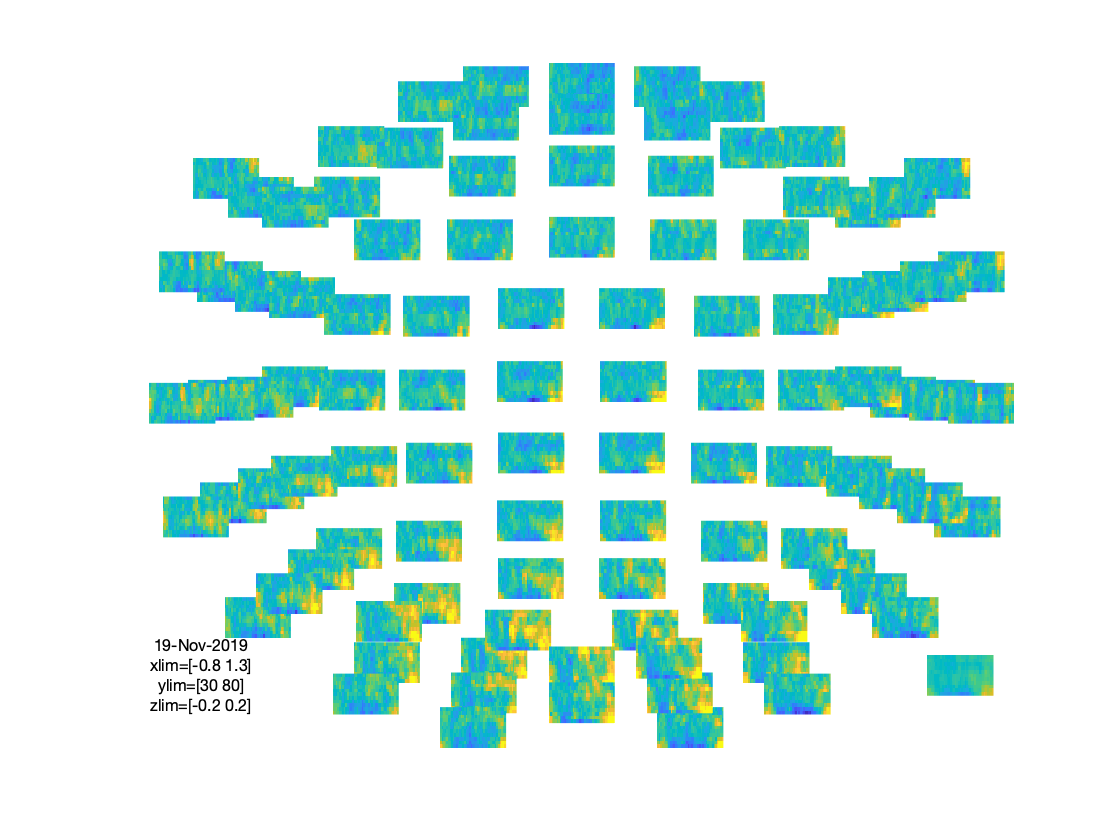
Figure: Time-frequency representations of power calculated using multitapers.
If you would like to learn more about plotting of time-frequency representations, please see the visualization section.
Exercise 5
Rather than visualising the TFRs in isolated conditions (after a baseline correction), you can also visualize the difference between 2 conditions, for example in the following way, using ft_math.
cfg = [];
cfg.parameter = 'powspctrm';
cfg.operation = 'log10(x1)-log10(x2)';
freqhigh_contrast = ft_math(cfg, freqhigh_famous, freqhigh_scrambled);
Inspect the resulting TFR, using interactive plotting. Note: don’t forget to NOT use the cfg.baseline and cfg.baselinetype options (why not?).
Time-frequency analysis IV
Morlet wavelets
An alternative to calculating TFRs with the multitaper method is to use Morlet wavelets. The approach is equivalent to calculating TFRs with time windows that depend on frequency using a taper with a Gaussian shape. The commands below illustrate how to do this. One crucial parameter to set is cfg.width. It determines the width of the wavelets in number of cycles. Making the value smaller will increase the temporal resolution at the expense of frequency resolution and vice versa. The spectral bandwidth at a given frequency F is equal to F/width2 (so, at 30 Hz and a width of 7, the spectral bandwidth is 30/72 = 8.6 Hz) while the wavelet duration is equal to width/F/pi (in this case, 7/30/pi = 0.074s = 74ms) (Tallon-Baudry and Bertrand (1999)).
Calculate TFRs using Morlet wavelet
cfg        = [];
cfg.method = 'wavelet';
cfg.output = 'pow';
cfg.foi    = 1:1:60;
cfg.width  = 7;
cfg.toi    = (-0.8:0.05:1.3);
cfg.pad    = 4;

cfg.trials = find(data.trialinfo(:,1)==1);
freq_famous = ft_freqanalysis(cfg, data);

cfg.trials = find(data.trialinfo(:,1)==2);
freq_unfamiliar = ft_freqanalysis(cfg, data);

cfg.trials = find(data.trialinfo(:,1)==3);
freq_scrambled = ft_freqanalysis(cfg, data);
Plot the result
cfg = [];
cfg.baseline     = [-0.6 -0.1];
cfg.baselinetype = 'absolute';
cfg.zlim         = [-1e-25 1e-25];
cfg.showlabels   = 'yes';
cfg.layout       = 'neuromag306mag_helmet.mat';
figure; ft_multiplotTFR(cfg, freq_famous)
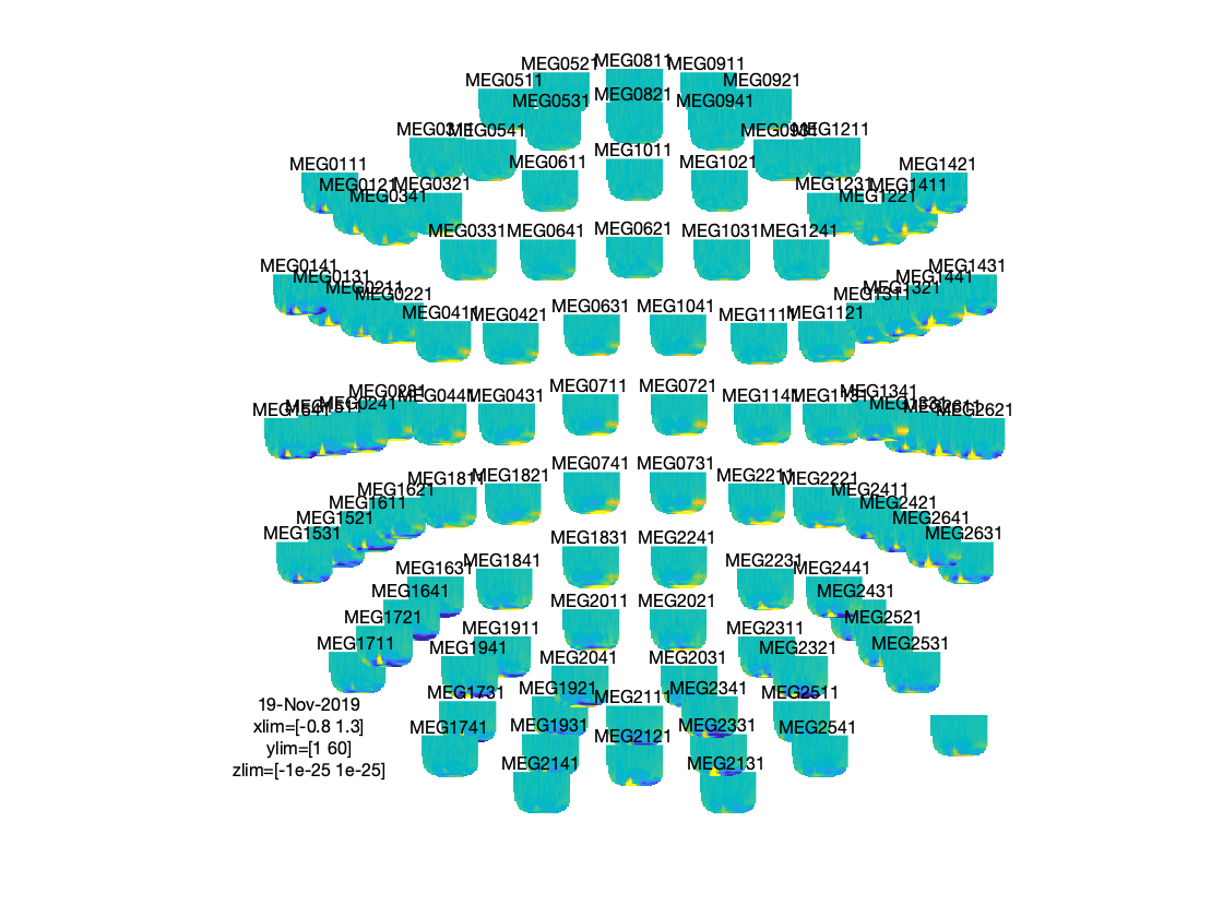
Figure: Time-frequency representations of power calculated using Morlet wavelets.
Exercise 6
Adjust cfg.width and see how the TFRs change.
If you would like to learn more about plotting of time-frequency representations, please see visualization.