The purpose of this page is just to serve as todo or scratch pad for the development project and to list and share some ideas.
After making changes to the code and/or documentation, this page should remain on the website as a reminder of what was done and how it was done. However, there is no guarantee that this page is updated in the end to reflect the final state of the project
So chances are that this page is considerably outdated and irrelevant. The notes here might not reflect the current state of the code, and you should not use this as serious documentation.
Testing minimum-norm estimate in FieldTrip and in MNE Suite
To test the equality of the two softwares solving the inverse solution with minimum-norm estimate we use a phantom data set from a 151 CTF MEG system.
Minimum-norm estimate in FieldTrip
Preprocessing
Here is the script that I use
cfg=[];
cfg.dataset='//MEG_phantom_CTF151/MagPhant_Phantom_20031211_01-av.ds';
cfg.trialdef.eventtype='?';
cfg=ft_definetrial(cfg);

% the following events were found in the datafile
% event type: 'STIM' with event values: 1  2  3  4  5  6  8
% event type: 'classification' with event values: 'Average' 'PlusMinus' 'StdDev'
% event type: 'frontpanel trigger' with event values: 8
% event type: 'trial' with event values:
% no trials have been defined yet, see FT_DEFINETRIAL for further help
% found 38 events
% created 0 trials


cfg = [];
cfg.dataset = '/<path>/MEG_phantom_CTF151/MagPhant_Phantom_20031211_01-av.ds';
cfg.trialdef.eventtype = 'trial';
cfg=ft_definetrial(cfg);

% cfg =
%
%          dataset: [1x10² char]
%         trialdef: [1x1 struct]
%      trackconfig: 'off'
%      checkconfig: 'loose'
%        checksize: 100000
%         datafile: [1x139 char]
%       headerfile: [1x139 char]
%       dataformat: 'ctf_meg4'
%     headerformat: 'ctf_res4'
%         trialfun: 'trialfun_general'
%            event: [38x1 struct]
%              trl: [3x3 double]
%          version: [1x1 struct]
I used only the first tria
cfg2 = cfg;
cfg2.trl = cfg.trl(1,:);

clear cfg;
cfg2.channel = 'MEG';
data=ft_preprocessing(cfg2);

data

% data =
%
%            hdr: [1x1 struct]
%          label: {151x1 cell}
%           time: {[1x600 double]}
%          trial: {[151x600 double]}
%        fsample: 600
%     sampleinfo: [1 600]
%           grad: [1x1 struct]
%            cfg: [1x1 struct]
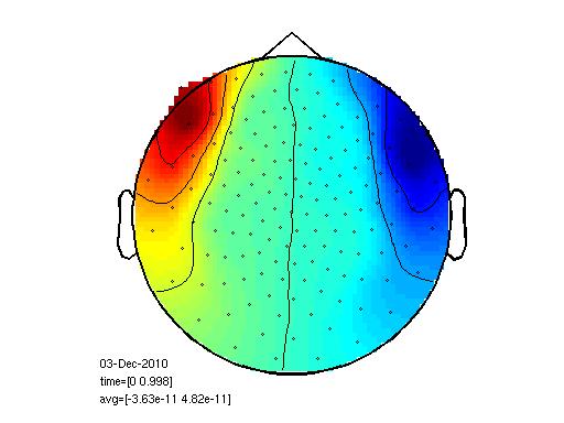
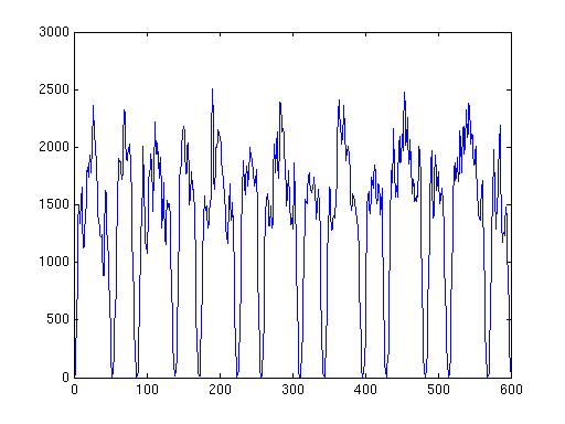
The data looks like this when I plot i
cfg=[];
topoplotER(cfg, data)
Averaging and Noise-covariance estimation
cfg  = [];
average = ft_timelockanalysis(cfg, data);
There is nothing to average indeed, because I use only one trial but I need to get the right structure from ft_timelockanalysis. The avg field of average and the trial field of data are indeed identical.
isequal(data.trial{1},average.avg)
It is evaluated to 1.
And I used this code for noise-covariance estimation. I defined the entire length as covariance window. I haven’t defined a baseline.
cfg = [];
cfg.latency = 'maxperlength';
cfg.keeptrials = 'yes';
cfg.covariance = 'yes';
cfg.channel = 'MEG';
cfg.covariancewindow = cfg.latency;
covariance = ft_timelockanalysis(cfg, data);

% covariance =
%
%         avg: [151x600 double]
%         var: [151x600 double]
%     fsample: 600
%        time: [1x600 double]
%         dof: [151x600 double]
%       label: {151x1 cell}
%       trial: [1x151x600 double]
%      dimord: 'rpt_chan_time'
%         cov: [1x151x151 double]
%        grad: [1x1 struct]
%         cfg: [1x1 struct]
It is not totally clear for me from the help why ‘keeptrials’ has to be yes. But I guess it is necessary for the noise-covariance estimation otherwise it makes an average from the data. It is written in the help that the default values of ‘latency’ is ‘maxperlength’ but I still had to define it.
Volume conductor
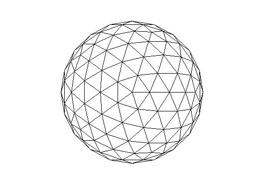
I created a sphere volume conductor with a 10 cm long radius.
vol_ph.r = 10;
vol_ph.o = [0,0,0];
vol_ph.c = 1;
vol_ph.type = 'singlesphere';
It looks like this (the function below creates a mesh out of it
ft_plot_headmodel(vol_ph)
Source space
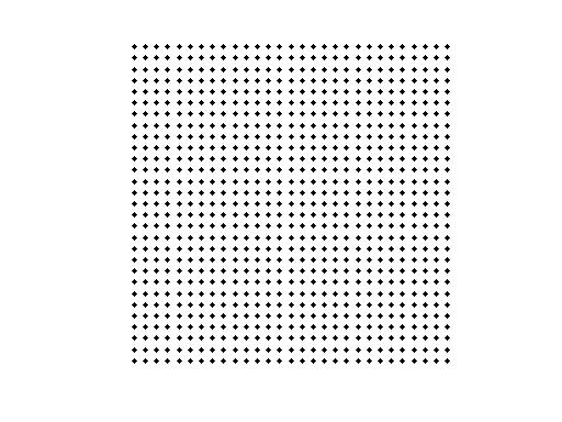
The source space is a 2D surface.
[X,Y]=ndgrid(-7:.5:7,-7:.5:7);
l = length(X(:)); %l = 841
pos = [X(:) Y(:) 7*ones(l,1)];


ft_plot_mesh(pos);
(This latest code does not work properly with an earlier version of MATLAB (MATLAB R2008b).)
Leadfield
cfg             = [];
cfg.grad        = data.grad;
cfg.headmodel   = vol_ph;
cfg.sourcemodel.pos    = pos;
cfg.channel     = 'MEG';
grid            = ft_prepare_leadfield(cfg);

% grid =
%
%           pos: [841x3 double]
%         tight: 'no'
%        inside: [641x1 double]
%       outside: [200x1 double]
%     leadfield: {1x841 cell}
%          cfg: [1x1 struct]
It is not clear for me when you have to define the option grid.inside and grid.outside at ft_prepare_leadfield.
Inverse solution
cfg=[];
cfg.headmodel = vol_ph;
cfg.grid = grid;
cfg.method = 'mne';
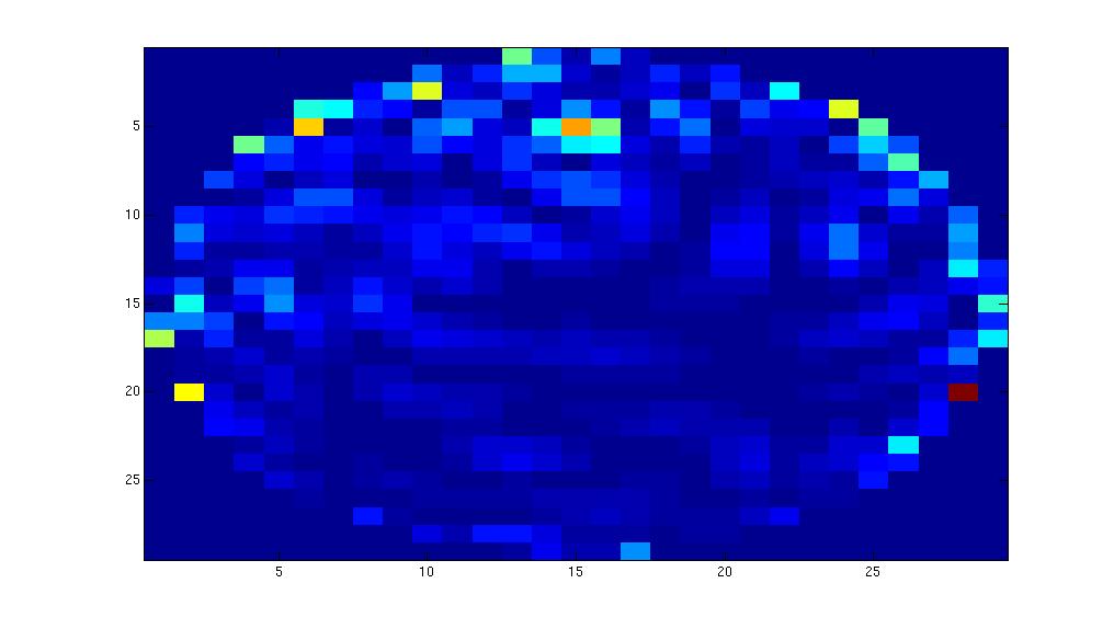
mne1 = ft_sourceanalysis(cfg,average);
figure;
mne1.avg.pow(100,30)
imagesc(reshape(mne1.avg.pow(:,30), 29,29))
Minimum-norm estimate in FieldTrip using simulated data
Trying to understand the results above, we looked at the phantom data in detail. It turned out that the location of the phantom with respect to the sensor-array was quite eccentric. To get a better idea about whether the results are caused by a feature of the code, or by the strange alignment we simulate some phantom data, where the active dipole is in the centre of the helmet.
cd ~jansch/matlab/toolboxes/fs2fieldtrip/
load grad;
load vol;
load grid;

figure;
ft_plot_sens(grad);
ft_plot_mesh(grid.pos);

cfg = [];
cfg.headmodel  = vol;
cfg.grad = grad;
cfg.channel = 'MEG';
cfg.dip.pos = [0 0 7];
cfg.dip.mom = [1 0 0];
cfg.dip.frequency = 10;
cfg.ntrials = 10;
cfg.triallength = 1;
cfg.fsample  = 1000;
cfg.relnoise = 0.01;
data = ft_dipolesimulation(cfg);
tlck = ft_timelockanalysis([], data);

cfg = [];
cfg.grid = grid;
cfg.headmodel  = vol;
cfg.grad = grad;
cfg.channel = 'MEG';
cfg.normalize = 'yes'; %depth normalization
grid = ft_prepare_leadfield(cfg);

cfg = [];
cfg.method = 'mne';
cfg.headmodel    = vol;
cfg.grid   = grid;
source = ft_sourceanalysis(cfg, tlck);
cfg.mne.noisecov = eye(151);
cfg.mne.lambda   = 0.01;
source2 = ft_sourceanalysis(cfg, tlck);

x = reshape(grid.pos(:,1), [29 29]);
y = reshape(grid.pos(:,2), [29 29]);
z = reshape(grid.pos(:,3), [29 29]);
figure;surf(x,y,z,reshape(mean(source.avg.pow,2), [29 29])); title('pinv');
figure;surf(x,y,z,reshape(mean(source2.avg.pow,2), [29 29])); title('no pinv');
This yields the following figure
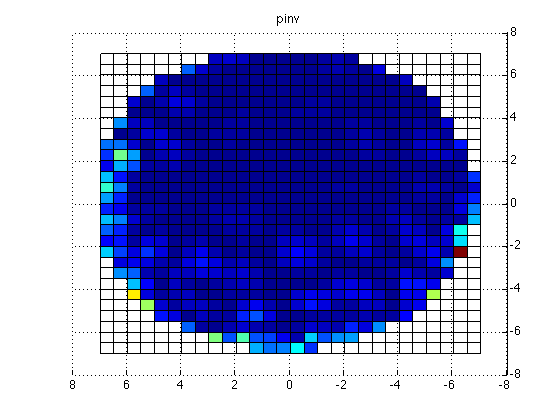
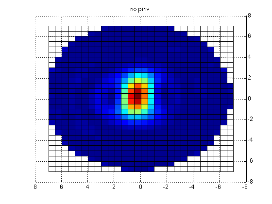
Clearly, there is an issue with the (default) pinv implementation. Apparently, some regularization should be done for the MNE to give meaningful results.
Back to the original phantom data, using FieldTrip and a regularized minimumnormestimate
Part 1.
This involves specifying cfg.mne.noisecov, cfg.mne.sourcecov, cfg.mne.lambda prior to calling ft_sourceanalysis.
cd ~jansch;
cfg.dataset = 'MagPhant_Phantom_20031211_01-av.ds';
hdr = ft_read_header(cfg.dataset);
cfg.trl = [1 600 0;601 1200 0;1201 1800 0];
cfg.channel = 'MEG';
data = ft_preprocessing(cfg);
% create volume conductor
vol = [];
vol.r = 7.5;
vol.o = [0 0 0];
vol.c = 1;
vol.type = 'singlesphere';
vol.unit = 'cm';
% create dipole grid
[X,Y,Z] = ndgrid(-7.5:0.25:7.5,-7.5:0.25:7.5,7);
grid = [];
grid.pos = [X(:) Y(:) Z(:)];
% compute leadfields
cfg = [];
cfg.grid = grid;
cfg.headmodel = vol;
cfg.grad = data.grad;
cfg.channel = 'MEG';
%cfg.normalize = 'yes';
grid = ft_prepare_leadfield(cfg);
% compute timelocked average
cfg = [];
cfg.trials = 1;
tlck = ft_timelockanalysis(cfg, data);
lf = cat(2,grid.leadfield{grid.inside});
for k = 1:size(lf,2)
n(k,1) = norm(lf(:,k));
end
n = reshape(n,[3 numel(n)/3]);
n = sum(n.^2);
n = repmat(n,[3 1]);
n = n(:);
% compute MNE
cfg = [];
cfg.method = 'mne';
cfg.headmodel = vol;
cfg.grid = grid;
cfg.mne.lambda = 1e-4; % trial and error
cfg.mne.noisecov = eye(151);
cfg.mne.sourcecov = spdiags(n.^-0.5, 0, numel(n), numel(n)); % this applies some depth weighting,
% the way it is described in the MNE manual
source = ft_sourceanalysis(cfg, tlck);
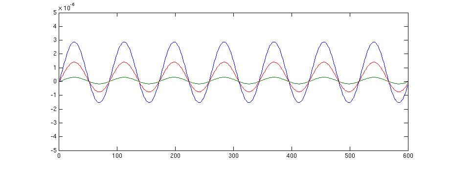
% plot a random source
figure;plot(source.avg.mom{source.inside(100)}');
This gives the following figur
% strange enough the data are not 0 mean
for k = 1:numel(source.inside)
indx = source.inside(k);
source.avg.mom{indx} = source.avg.mom{indx} - repmat(mean(source.avg.mom{indx},2), [1 size(source.avg.mom{indx},2)]);
end

% project source activity onto the dominant orientation
cfg            = [];
cfg.projectmom = 'yes';
sd             = ft_sourcedescriptives(cfg, source);

m = zeros(3721,600);
m(sd.inside,:) = cat(1,sd.avg.mom{sd.inside});
m = sqrt(sum(m.^2,2));
m(m==0)=nan;

bnd = [];
bnd.pnt = source.pos;

[az,el,r] = cart2sph(bnd.pnt(:,1),bnd.pnt(:,2),bnd.pnt(:,3));
[x, y]    = pol2cart(az, pi/2 - el);
proj      = [x y];
bnd.tri   = delaunay(x, y);

figure;hold on;
ft_plot_mesh(bnd,'vertexcolor',m,'edgecolor','none');axis on
Part 2.
Now, I do the same as above (part 1.) but I use the same volume conductor and grid as what I used for MNE Suite.
%cd ~jansch;
cfg.dataset = '/home/language/lilmag/phantom data/MagPhant_Phantom_20031211_01-av.ds';
hdr         = ft_read_header(cfg.dataset);
cfg.trl     = [1 600 0;601 1200 0;1201 1800 0];
cfg.channel = 'MEG';
data        = ft_preprocessing(cfg);

% create volume conductor
vol   = [];
%vol.r = 7.5;
vol.r = 10;
vol.o = [0 0 0];
vol.c = 1;
vol.type = 'singlesphere';
vol.unit = 'cm';

% create dipole grid
%[X,Y,Z]  = ndgrid(-7.5:0.25:7.5,-7.5:0.25:7.5,7);
[X,Y]=ndgrid(-7:.5:7,-7:.5:7);
l = length(X(:)); %l = 841

grid     = [];
%grid.pos = [X(:) Y(:) Z(:)];
grid.pos = [X(:) Y(:) 7*ones(l,1)];

% compute leadfields
cfg      = [];
cfg.grid = grid;
cfg.headmodel  = vol;
cfg.grad = data.grad;
cfg.channel = 'MEG';
%cfg.normalize = 'yes';
grid     = ft_prepare_leadfield(cfg);

% compute timelocked average
cfg  = [];
cfg.trials = 1;
tlck = ft_timelockanalysis(cfg, data);

lf = cat(2,grid.leadfield{grid.inside});
for k = 1:size(lf,2)
n(k,1) = norm(lf(:,k));
end
n = reshape(n,[3 numel(n)/3]);
n = sum(n.^2);
n = repmat(n,[3 1]);
n = n(:);

% compute MNE
cfg        = [];
cfg.method = 'mne';
cfg.headmodel    = vol;
cfg.grid   = grid;
cfg.mne.lambda    = 1e-4; % trial and error
cfg.mne.noisecov  = eye(151);
cfg.mne.sourcecov = spdiags(n.^-0.5, 0, numel(n), numel(n)); % this applies some depth weighting,
% the way it is described in the MNE manual
source            = ft_sourceanalysis(cfg, tlck);

% plot a random source
figure;plot(source.avg.mom{source.inside(100)}');
% strange enough the data are not 0 mean
for k = 1:numel(source.inside)
indx = source.inside(k);
source.avg.mom{indx} = source.avg.mom{indx} - repmat(mean(source.avg.mom{indx},2), [1 size(source.avg.mom{indx},2)]);
end

% project source activity onto the dominant orientation
cfg            = [];
cfg.projectmom = 'yes';
sd             = ft_sourcedescriptives(cfg, source);

%m = zeros(3721,600); %why is this 3721? source.dim, pos
m = zeros(841,600);
m(sd.inside,:) = cat(1,sd.avg.mom{sd.inside});
m = sqrt(sum(m.^2,2));
m(m==0)=nan;

bnd = [];
bnd.pnt = source.pos;

[az,el,r] = cart2sph(bnd.pnt(:,1),bnd.pnt(:,2),bnd.pnt(:,3));
[x, y]    = pol2cart(az, pi/2 - el);
proj      = [x y];
bnd.tri   = delaunay(x, y);

figure;hold on;
ft_plot_mesh(bnd,'vertexcolor',m,'edgecolor','none');axis on
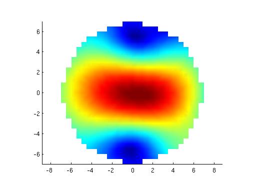
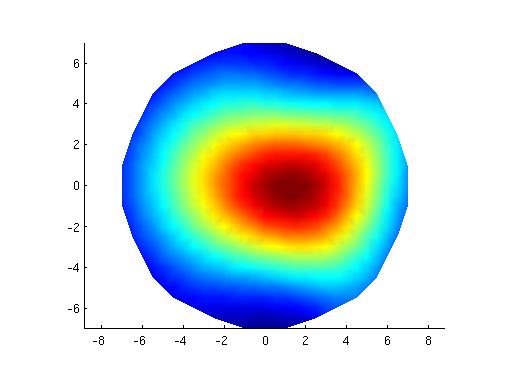
I have also tried to plot it the same way as I plot the mesh for the MNE suite results (see below). And I changed lambda to 0.01 (because 0.01^2 = 1e-4).
[r,c]=find(source.avg.pow==max(source.avg.pow(:)))
%max at 198.
m = source.avg.pow(:,198);
spoints = source.inside;
bnd = [];
%bnd.pnt = source.pos;
bnd.pnt = source.pos(spoints,:);
mred = m(spoints,:);
[az,el,r] = cart2sph(bnd.pnt(:,1),bnd.pnt(:,2),bnd.pnt(:,3));
[x, y] = pol2cart(az, pi/2 - el);
proj = [x y];
bnd.tri = delaunay(x, y);
figure;hold on;
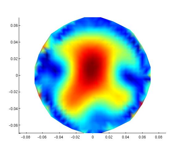
ft_plot_mesh(bnd,'vertexcolor',mred,'edgecolor','none');axis on
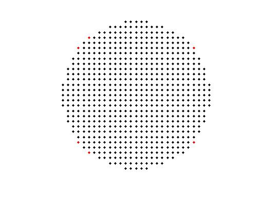
Part 3.
Now, I will use the leadfield from the MNE Suite analysis of the phantom data.
%%%%%
%% load forward solutions
%%%%%

% the forward solution from MNE Suite
fwd = mne_read_forward_solution('/<path>/test_phantom/MEG/phantomas/phantomas-fwd.fif');

% the leadfield from FieldTrip (see above)
load grid;

size(grid.inside,1)

% 641

size(fwd.source_rr,1)

% 635

% the number of source points for which the forward solution was calculated is not equal

%%%%%
%% make same source space
%%%%%

% look for the points that are different (e.g., missing from the MNE suite fwd)

vertno = fwd.src.vertno; % this contains the indices of the used source points
v_st = int2str(vertno');
g_st = int2str(grid.inside);
sameind = [];

k=length(v_st); %635

for i=1:k
  x = 0;
  x = strmatch(v_st(i,:),g_st,'exact');
  if isempty(x) == 0
  sameind(i)=x;
  end

end

% sameind shows which rows of grid.inside contains common source points indexes
% missing from sameind: 32, 72, 94, 548, 570, 592

missind = [32, 72, 94, 548, 570, 592];

gridnew = grid.inside(sameind,:); %this are the indices that are present in vertno
griddiff = grid.inside(missind,:); %this are the indices that are not present in vertno

% plot the new grid with the missing points in different color (red)

ft_plot_mesh(grid.pos(griddiff,:), 'vertexcolor', 'red');
hold on;
ft_plot_mesh(grid.pos(gridnew,:));
grid2 = grid;
grid2.inside = grid.inside(sameind,:);
grid2.outside = sort([grid2.outside; grid.inside(missind,:)]);

isequal(grid2.inside,fwd.src.vertno')

% ans =
%
%      1

%delete forward solution for source points that won't be used

grid2.leadfield{grid.inside(missind(1))} = NaN;
grid2.leadfield{grid.inside(missind(2))} = NaN;
grid2.leadfield{grid.inside(missind(3))} = NaN;
grid2.leadfield{grid.inside(missind(4))} = NaN;
grid2.leadfield{grid.inside(missind(5))} = NaN;
grid2.leadfield{grid.inside(missind(6))} = NaN;

%%%%%
%% make new leadfield
%%%%%

% I substitute the leadfield values of the FT grid with the MNE Suite solution and I swap the x % and y dimensions

l = length(grid2.inside);

for i=1:l
  data = fwd.sol.data(:,(1:3)+(i-1)*3);
  data2 = cat(2, data(:,2), data(:,1), data(:,3));
  grid2.leadfield{grid2.inside(i)}=data2;
end
FIXME I should match the positions of the source points with each other.
%%%%%
%% source-analysis
%%%%
load tlck; % see above
load vol; % see above
lf = cat(2,grid2.leadfield{grid2.inside});
for k = 1:size(lf,2)
n(k,1) = norm(lf(:,k));
end
n = reshape(n,[3 numel(n)/3]);
n = sum(n.^2);
n = repmat(n,[3 1]);
n = n(:);
% compute MNE
cfg = [];
cfg.method = 'mne';
cfg.headmodel = vol;
cfg.grid = grid2;
%cfg.mne.lambda = 1e-4; % trial and error
cfg.mne.lambda = 0.01; %1e-4^2=0.01
cfg.mne.noisecov = eye(151);
cfg.mne.sourcecov = spdiags(n.^-0.5, 0, numel(n), numel(n));
% this applies some depth weighting, the way it is described in the MNE manual
source2 = ft_sourceanalysis(cfg, tlck);
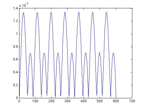
% plot a random source
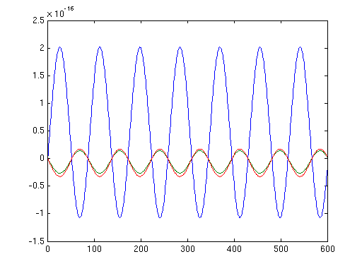
figure;plot(source2.avg.mom{source2.inside(100)}');
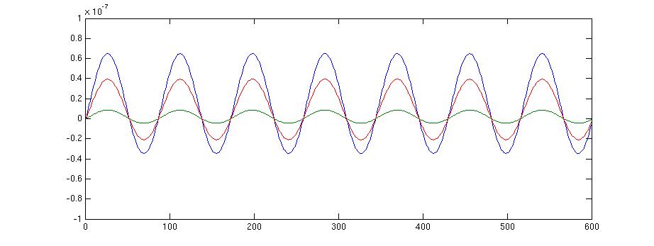
The same figure of a random source calculated with the original leadfield of FieldTrip looks like this:
Note, that the values in the second figure are much larger.
%%%%%
%% plot the result
%%%%%
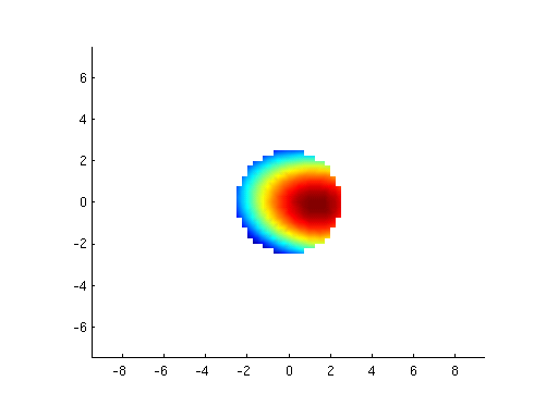
% look for the largest value
[r,c]=find(source3.avg.pow==max(source3.avg.pow(:)))
%max at 284. (upps, it was max also at 284 for the MNE result)
m = source2.avg.pow(:,284);
spoints = source2.inside;
mred = m(spoints,:);
bnd = [];
%bnd.pnt = source.pos;
bnd.pnt = source2.pos(spoints,:);
[az,el,r] = cart2sph(bnd.pnt(:,1),bnd.pnt(:,2),bnd.pnt(:,3));
[x, y] = pol2cart(az, pi/2 - el);
proj = [x y];
bnd.tri = delaunay(x, y);
figure;hold on;
ft_plot_mesh(bnd,'vertexcolor',mred,'edgecolor','none');axis on
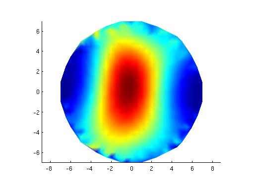
Compare this to figure at the end of the next session (“Minimum-norm estimate with MNE Suite using phantom data”).
Minimum-norm estimate in MNE Suite using phantom data
Setting up the environmental variables and etc.
export MNE_ROOT=/<path>/MNE/MNE-2.7.0-3106-Linux-x86_64
echo $MNE_ROOT
export MATLAB_ROOT=/<path>/matlab
cd $MNE_ROOT/bin
. ./mne_setup_sh export SUBJECTS_DIR=/data/corpora/MPI_workspace/ncl/studass/lilla/FT/test/subjects echo $SUBJECTS_DIR export SUBJECT=phantomas
Data conversion
cd /<path>/test/MEG/phantomas
mne_ctf2fiff --ds MagPhant_Phantom_20031211_01-av.ds --fif phantomas-raw
Setup source space
First, I have created text files with matlab.
pos_mm=pos.*10; %this pos structure is the same that I used in FT


fid = fopen('pos.txt', 'wt');
n=size(pos_mm,1);
for line = 1:n
  num = pos_mm(line,1);
  fprintf(fid, '%-1.0f ',num);
  num = pos_mm(line,2);
  fprintf(fid, '%-1.0f ',num);
  num = pos_mm(line,3);
  fprintf(fid, '%-1.0f\n',num);

end
fclose(fid);
And then, I created the source space for MNE Suite.
mne_volume_source_space --pos /<path>/pos.txt --src /<path>/test/subjects/phantomas/bem/phantomas-src.fif
Creating the volume-conductor
First, I have created a text file in MATLAB with .tri extension
clear all;
[pnt, tri]=icosahedron642;
pnt_mm=pnt.*100; %10cm = 100 mm;
fid = fopen('vol1.txt', 'wt');
n=size(pnt_mm,1);
fprintf(fid, '%-1.0f\n',n);
for line = 1:n
  num=pnt_mm(line,1);
  fprintf(fid,'%g ', num);
  num = pnt_mm(line,2);
  fprintf(fid, '%g ',num);
  num = pnt_mm(line,3);
  fprintf(fid, '%g\n',num);

end
n=size(tri,1);
fprintf(fid, '%-1.0f\n',n);
for line = 1:n
  num=tri(line,1);
  fprintf(fid,'%-1.0f ', num);
  num = tri(line,2);
  fprintf(fid, '%-1.0f ',num);
  num = tri(line,3);
  fprintf(fid, '%-1.0f\n',num);

end
fclose(fid);
I renamed the .txt file to .tri. And then, I used MNE Suite.
mne_surf2bem --tri /<path>/vol.tri --sigma 1 --id 1 --fif /<path>/test/subjects/phantomas/bem/phantomas-bem.fif
:?: The value (1) after sigma is the conductivity value that is supposed to be in S/m. I set it to 1 because conductivity was set to 1 also in FT, but I do not know the unit of the conductivity in FT. The value (1) after id means that this is an innerskull mesh. I do not know if it is necessary to specify this.
Averaging
I had to rename phantomas-raw.fif to phantomas_raw.fif.
cd /data/corpora/MPI_workspace/ncl/studass/lilla/FT/test/MEG/phantomas
mne_browse_raw
File… Open…
Compensation:Third-order gradient, Selection: phantomas_raw.fif
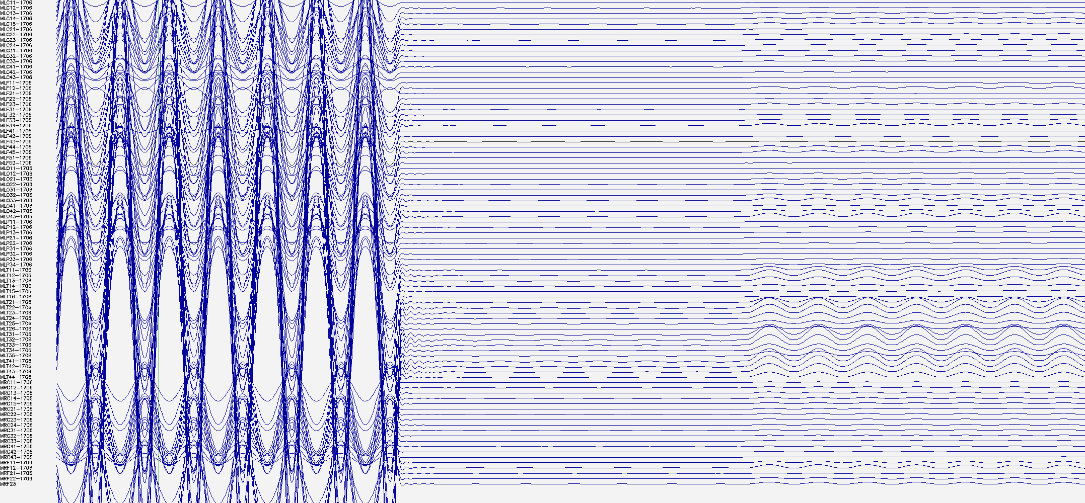
To look at the data in topographical vie
Adjust… Full view layout… CTF-151 Windows… Show full view
I had to create a new event list in a text editor
0 0.000        0   0
600 1.000        0   1
Saved as phantomas1.eve.
I did the averaging in batch mode with the help of an averaging file.
mne_process_raw --raw phantomas_raw.fif --projoff --filteroff --events phantomas1.eve --ave phantomas.ave --digtrig STIM
The averaging file (phantomas.ave
average {
#
Output files
#
outfile         phantom-ave.fif
logfile         phantom-ave.log
eventfile  phantom1-eve.fif
Category specifications
#
category {
  name  "trial"
  event  1
  tmin  -1
  tmax  0
  color  1 1 0
}
}
(I haven’t rejected anything and there is no baseline.)
Back to MNE browser to look at the averages.
mne_browse_raw
File… Open evoked Selection: phanotmas-ave.fif To se Adjust… Full view layout… CTF-151 Windows.. Show averages (If amplitude is to big: Adjust… Scales… Scale magnification for averages: 0.1)
To look at how many trial Windows… Manage averages… (It should be N=1)
Noise-covariance matrix estimation
I made a noise-covariance matrix in MATLAB. It was necessary because MNE did not calculate a noise-covariance matrix because I had only 1 trial that is shorter than 20 s.
cov = [];
cov.data = eye(186);

cov.kind = 1; %1 = noise covariance

cov.dim = 186; %dimension of the covariance matrix

cov.nfree = []; %this becomes -1

rawinfo = fiff_read_meas_info('/<path>/phantomas_raw.fif');
cov.names = rawinfo.ch_names;

cov.diag = 0; %this is not a diagonal matrix

cov.eig = [];
cov.projs = [];
cov.bads = [];

mne_write_cov_file('phantomas3-cov.fif',cov);
Coordinate alignment
mne_analyze
I haven’t aligned anything but a transformation matrix saved (with diagonal matrix with 1’s on the diagonal).
Forward solution
mne_prepare_bem_model --bem /<path>/test/subjects/phantomas/bem/phantomas-bem.fif --sol /<path>/test/subjects/phantomas/bem/phantomas-bem-sol.fif --method linear

mne_do_forward_solution --src phantomas-src.fif --bem phantomas-bem.fif  --meas phantomas-ave.fif --fwd phantomas-fwd.fif --megonly
Inverse solution
mne_do_inverse_operator --fwd phantomas-fwd.fif --senscov phantomas3-cov.fif --meg
Visualizing the result in MATLAB
res = mne_ex_compute_inverse('/home/language/lilmag/Lilla/phantom_mne/phantomas-ave.fif',1,'/home/language/lilmag/Lilla/phantom_mne/phantomas-meg-inv.fif',1,1e-4,[]);
The arguments ar
fname_data - Name of the data file
setno - Data set number
fname_inv - Inverse operator file name
nave - Number of averages (scales the noise covariance) If negative, the number of averages in the data will be used
lambda2 - The regularization factor
dSPM - do dSPM?
I got a res structure.
figure; plot(res.sol(100,:));
[r,c]=find(res.sol==max(res.sol(:)))
Maximum was at 284.
m = res.sol(:,284);

spoints = res.inv.src.inuse;
z = find(spoints == 1);

bnd = [];
m = res.sol(:,284);


spoints = res.inv.src.inuse;
z = find(spoints == 1);

bnd = [];
%bnd.pnt = source.pos;
bnd.pnt = res.inv.src.rr(z,:);


[az,el,r] = cart2sph(bnd.pnt(:,1),bnd.pnt(:,2),bnd.pnt(:,3));
[x, y]    = pol2cart(az, pi/2 - el);
proj      = [x y];
bnd.tri   = delaunay(x, y);

figure;hold on;
ft_plot_mesh(bnd,'vertexcolor',m,'edgecolor','none');axis on