FieldTrip Walkthrough

Foreword

This walkthrough is intended to give a little background in the use of FieldTrip. It is not a manual, nor is it meant to be canonical or generic for all possible uses. I am making this from my limited experience as a user, not as a developer. Also, at the time of making this, many modifications on the code, both in detail as well as more substantive ones (e.g., a different implementation of data structure in its main functions) are planned. I do believe, however, that an absolute beginner might benefit from a bit of overview, especially those who want to end up using FieldTrip for frequency and time-locked (MEG) data-analysis within a cognitive paradigm in humans, from sensor to source level. It is meant to be read before one commences with the analysis as a background on which to explore the already detailed documentation available at the FieldTrip website. However, some experience in programming, and of MATLAB in particular, is definitely needed. I would like to refer to the MATLAB knowledge database on intranet for those that need help getting started (at the Donders Center). Finally, please see this attempt itself as experimental. Because of the fact that FieldTrip, from the developers point of view, is investing most of its efforts in innovation, a full manual will never be up to date, or even correct, at least not for long.

Happy FieldTripping, Stephen Whitmarsh

Trial based analysis

Introduction

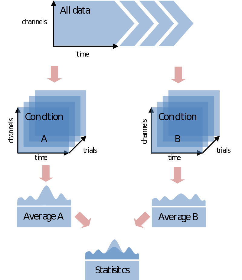
In most cases you would like to analyze your data in respect to stimulus/condition markers recorded within the data. Alternatively, you might want to define trials based upon visual inspection of the data, or based upon recordings of external device (eye-tracker, EOG, SCR, TMS, etc) or log file. For the sake of the purpose of overview only go into the first option although all these latter options are certainly supported in FieldTrip. If possible always record stimulus/condition markers in your EEG/MEG data. It will make the analysis, if not life itself, substantially easier. You might have coded every stimulus with its own code, or rather used the marker to code the condition number. In any case, most probably the first step you want to do is to load your data and segment it into conditions according to the markers in the data. In the end you’ll just need to find a nice test-statistic, e.g., average alpha-power, and do your statistical comparison:

Data Structure in FieldTrip

First of all it is very important to get comfortable with the way FieldTrip manages the structure of your data. Although it might take a little getting used to, in many ways it is obvious and determined by the inherent structure of the data. EEG and MEG data is composed of many channels and many time points. Therefore it contains a sample, a single number representing microvolts or femtoteslas, for every Channel x Time point:

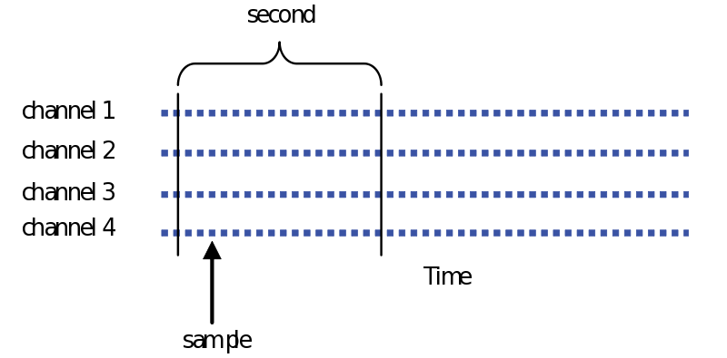
In Fieldtrip this is contained within in a single data matrix of [channels x timepoints], for instance:

data.trial{1}: [32x1000 double]

For now you can ignore that fact that it is within a field called ‘trial’. At the moment there is only one trial so this is just to be able to generalize to the case then we have segmented the data into separate trials. So if you, for instance, want to refer to the 10th sample of the second channel, you might simply type

data.trial{1}(2,10)

Note that the exact timing can’t be derived from the data itself. For that we need to know the sample rate (in samples per second, or Hertz). This is found in the data structure as an extra field called ‘fsample’. For example:

data.fsample = 600;

The representation of the data in terms of time is of course relative. In most cases only after defining trials will we be saying something like “at 0.5 seconds after stimulus”.

Trial structure

Similar to how the inherent structure of the original data is represented in the first step described above, the trial structure is also implemented at the level of the data structure. This means that if you cut up your data into separate trials, the new structure of the data will reflect this. The added dimension of trials is represented in FieldTrip as a series of [channels x time] cell-arrays:

data.trial: {1x25 cell}

Looking at one trial separately gives us the familiar channels x time structure:

data.trial{5}: [32x1000 double]

Most often every trial has the same time axis. e.g., they all go from one second before the marker until three second after the marker. This is not always the case however, and this is why every trial has its own time axis. It has the same length as the data, defining a (relative) time point in seconds for every sample in the data, for instance:

data.time{5}: [1x1000 double]    % of which a small part might be:  [… 1.06 1.07 1.08 1.09 …]

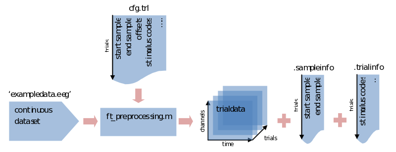
Where the trials were originally from, meaning the samples in the continuous data are found in data.sampleinfo. It has a simple two column format of a start and end sample number for every trial (on every row).

data.sampleinfo: [2x25 double]   % one row might be: [173450 174450]

Finally, you might have extra information per trial about the specific condition to which the trial belongs, the response time, etc. How to include this information yourself will be explored next but for now it will suffice to say you can might find it in an extra field called trialinfo where every row contains some extra info for every trial. For example:

data.trialinfo: [3x25 double]    % one row might be: [100 3.4556 1] 

Trial bookkeeping, part I

At this point you might ask: “how does FieldTrip know which trials correspond to which condition?” Unlike perhaps other analysis packages, it doesn’t. You will have to do your own bookkeeping on that. How you want to do that, and indeed if you want to do that, will depend on how you want to undertake your analysis. Let’s take the simplest case of comparing the averages (or whatever) of two conditions. In FieldTrip this can be done in two ways:

• Doing the whole analysis separately for each condition (starting with preprocessing).
• Average over conditions
• Compare the averages

or

• Doing the whole analysis over all the trials at once.
• Split the trials belonging to each condition.
• Average over conditions
• Compare the averages

The main difference between the two approaches considering trial bookkeeping is that in the first case you do not need any trial bookkeeping – you simply only read and process the data you need separately for every conditions. The other option is to postpone the separation of trials into conditions. This would make sense in any trial-by-trial based analysis [sic] or just purely for the sake of keeping stuff together. We’ll start with the first step. The second is an extension of that one.

Defining trials

Assuming we have marked our data file with codes representing conditions, we want to know how to segment the data relative to these markers. Note that although you might only be interested in the first second after the stimulus code, you might want to consider including a baseline period. Of course there are many other considerations. For the moment we will assume all trials to be of equal length and not to be overlapping.

So first of all we need to specify what marker codes belongs to what condition. We do that by creating two arrays of codes, one for every condition, e.g.

markersA = [1:5 11];                        % 1 2 3 4 5 11
markersB = [6:10 12];                       % 6 7 8 9 10 12

Then there is the timing we need to define. Let’s already put it in a cfg structure (more about the cfg structure later):

cfg = [];                                   % create an empty variable called cfg
cfg.trialdef.prestim = 0.5;                 % in seconds
cfg.trialdef.poststim = 2;                  % in seconds

In addition, we need to specify where those markers are located. This will be different for every system.

cfg.trialdef.eventtype = 'input';           % use '?' to get a list of the available types

Let’s now also add to the cfg the events as we specified them a moment before and - as we decided previously - one condition at a tim

cfg.trialdef.eventvalue = markersA;

Now, the last thing we need to do is to point to the datafile where to read the event markers from.

cfg.dataset = 'subject01.eeg';

We can now call our first FieldTrip function

cfg = ft_definetrial(cfg);

Notice that what is happening here is that a cfg structure is fed into ft_definetrial, which returns it again but with an added field called cfg.trl. This is a simple list of three columns where every row describes a separate trial start, end and offset (interval before the event) in sample numbers, relative to the event values we specified

cfg.trl: [50x3 double]

This is all we need to load the appropriate data using ft_preprocessing, using the different stimulus events values to load every condition separately. You can jump ahead to preprocessing or stay for the next part where we will look at how to adapt our trial definition so we can still do some trial bookkeeping later on.

Trial bookkeeping, part II

What makes ft_definetrial very flexible is that it uses a separate trial function you can customize to fit your specific requirements.

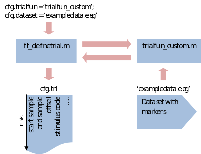
Within trialfun the trl is made according to specifications given through the cfg, as well as anything else you want to add. For instance, you might want to make trials dependent not only on the stimulus marker, but also on a correct response marker. This would be the place to do that. Also, sometimes you might be left with a rather awkward way of coding your conditions. This would also be the place to recode your trials and create a less ambiguous system. For the purpose of trial bookkeeping we only need to append one extra column (or more) to the standard three columns of the trl. Here we write information about the stimulus code, response time, condition numbers, etc. Next in ft_preprocessing (explained next) these extra columns will be put in an extra field of the data structure (trialinfo). This will enable us at any moment during our analysis to select trials based upon any arbitrary reason.

Preprocessing

Preprocessing (ft_preprocessing.m) was the second main function implemented during FieldTrip’s development. As the name suggests it’s takes care of the first steps in processing your data. This means, including (but certainly not restricted to

1. Loading the data into a FieldTrip data structure
2. Rereferencing
3. Cutting up your data into trials (if a trl is specified)
4. Baseline correction
5. Detrend
6. Filtering (high, low, band pass and notch)

Besides loading the data all the other functionalities can be done at any later stage. They are not set by default. We’ll go through them in their own time and use ft_preprocessing only for the first two steps.

If we don’t specify the trial definition we made previously, ft_preprocessing would load all data and put them into a [channels x time] array of a single trial (e.g., in data.trial{1}). To save memory it is sometimes preferred to load only the data that is actually used, and you’ll need to segment the data into trials sooner or later anyway. To do so we supply ft_preprocessing with the trl we made previously. You might have everything you need already specified within the cfg, but just to be sure we’ll repeat it here:

cfg.trl = trl;                      % saved somewhere previously
cfg.dataset = 'exampledata.eeg';    % data file, you might also need to add the path to it
trialdata = ft_preprocessing(cfg);  % call preprocessing, putting the output in 'trialdata'

What we end up with now is a datastructure called trialdata. See the previous ‘trialstructure’ on how the data it is organized. Please note here that all the info that was contained in the trl is now put in two different fields of the datastructure. The first two colums of the trl that described the start and end samples in the original data are now found in trialdata.sampleinfo. All the extra information for our trial bookkeeping that was put in extra columns of the trl are now found in trialdata.trialinfo.

Artifact rejection

Introduction

Finding an appropriate approach to artifact rejection is not as simple as one might think. Every system, every experiment and even every subject will vary in number, magnitude and type of artifacts. Also, some researchers might be okay with just rejecting trials with any artifacts, some only if eye blinks come before a stimulus, while again others might want to correct for eye and movement artifacts by using an ICA approach. Furthermore, some artifacts, like spikes, might be easy to detect because of their signal properties, while others might be much harder to detect. For these reasons I believe one cannot do without visual inspection of the data. Only in very rare cases of very typical and well described artifacts, such as jumps from a specific MEG system, we think a full automatic artifact rejection is warranted. Besides all those rational considerations, manually going through your data early will also give you a certain ‘feeling’ of what your data is like.

Of course, in the end you would like to have certain standardized approach to your artifact rejection that will give you the best results possible. I don’t know if something like that exists and rather think everyone has his or her own personal preferences. Although seemingly rather time-consuming, I myself ended up with the following procedure. You need not follow it, it’s just a suggestion. It does give me the possibility of explaining some of the following steps in more detail. In particular it will explain a use of ft_databrowser, a recently added function which is not yet documented elsewhere.

1. Visually inspect the dataset and mark those segments that contain obvious movements, (system) spikes or muscle artifacts, leaving in all but the most extreme eye artifacts.
2. Reject the trials that contain artifacts.
3. Decompose the data using ICA. Note that ICA can give very unreliable results when the data contains a lot of (correlated) noise. The cleaner the data is already, the better the ICA results.
4. Find components clearly corresponding to eye blinks and saccades.
5. Recompose data without those components.
6. Go through data again visually and manually selects segments that still show any remaining artifacts, being from eye blinks, movements, etc.

I know this looks like a lot of work. However, it might pay off in the end when you are certain your data is clean and you do not have to go back to satisfy that slightly uneasy feeling that your results might ‘be all artifacts’. Of course they might still be, but at least you did everything you could.

Visual data inspection

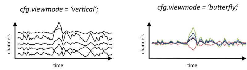
As most FieldTrip functions ft_databrowser needs a configuration structure and a data structure as input. First of all we can specify how to visualize the data:

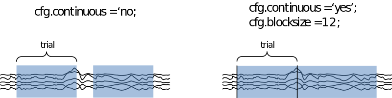
We can also specify if we want to look at the data trial-by-trial, or if we want to treat it as continuous data. In the latter case we need to specify how large the time segments on display need to be in cfg.blocksize (in seconds

If we now call ‘‘cfg = ft_databrowser(cfg,data)’’, we are able to scroll through the data and select those segments containing muscle artifacts and the like. In the case you want to remove eye artifacts with ICA you can leave those in. If we now exit the databrowser by pressing ‘q’ our cfg is returned with an extra field containing a list of start and end samples for every data segment we selected

cfg.artfctdef.visual.artifact: [2xnArtifacts double]

Note that ft_databrowser does not do anything with your data. To remove the trials that overlap with the segments we selected (and which are now in our cfg) and to save the remaining data in a new data structure we still need to use the function ft_rejectartifact:

cfg.artfctdef.reject  = 'complete';
cleandata = ft_rejectartifact(cfg,data);

Using ICA for eye artifact removal

Severe contamination of EEG/MEG activity by eye movements, blinks, muscle, heart and line noise is a serious problem for its interpretation and analysis. Many methods exist to remove eye movement and blink artifacts. Simply rejecting contaminated epochs results in a considerable loss of collected information. Often regression in the time or frequency domain is performed on simultaneous electro-oculographic (EOG) recordings to derive parameters characterizing the appearance and spread of EOG artifacts in the other channels. However, EOG records also contain brain signals, so regressing out EOG activity inevitably involves subtracting a portion of the relevant brain-signal from each recording as well. Also, since many noise sources, include muscle noise, electrode noise and line noise, have no clear reference channels, regression methods cannot be used to removed them. ICA can effectively detect, separate and remove activity in EEG/MEG records from a wide variety of artifactual sources, with results comparing favorably to those obtained using regression- or PCA-based methods (http://sccn.ucsd.edu/~scott/tutorial/).

First we need to decompose the data into independent components. The only thing we have to be sure of is that we only use the actual EEG or MEG channels and don’t use reference sensors or EOG:

cfg = \[];
cfg.channel = 'EEG';
ic_data = ft_componentanalysis(cfg, cleandata);

The ICA will return as many components as you put channels in. Each component consists of a component time course for every trial (ic_data.trial) together with a single topography (ic_data.topo

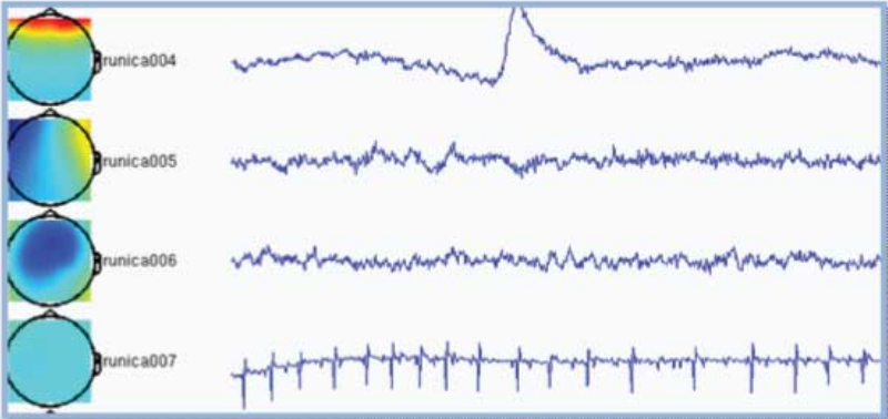
When ft_componentanalysis is done (it could take a while) we have to find those components we want to subtract from our data. We’ll use ft_databrowser for this again, only looking at ten ‘channels’ (components) at a time:

cfg = [];
cfg.viewmode = 'component';
cfg.continuous = 'yes';
cfg.blocksize = 30;
cfg.channels = [1:10];
ft_databrowser(cfg, ic_data); 

Components are automatically sorted based upon on the sum of the weighting factors, commonly resulting in the most interesting components appearing on top. In the example below the first component is clearly an eye-blink because the appearance of an eye-blink in the time-course and the frontal topography. The second component is most probably related to eye movements for similar reasons. The fourth component is picking up the heartbeat. There is no reason to assume the third component to be artifactual.

To recompose the data without components 1, 2 and 4 use ft_rejectcomponent

cfg = [];
cfg.component = [1 2 4];
data_iccleaned = ft_rejectcomponent(cfg, ic_data);

Our data is quite clean now but I would recommend a last manual inspection on a trial by trial basis. It might happen that you missed some artifacts in the first run as it was only a rough scan for the benefit of the ICA. It might also very well be that the ICA failed for some reason, or that you skipped artifacts in the first run that you thought were eye-blinks but which were not removed in the end. Although you know the drill by now, here is the code:

cfg = [];
cfg.viewmode = 'horizontal';
cfg.continuous = 'no';
ft_databrowser(cfg,data_iccleaned);

cfg.artfctdef.remove = 'complete';
data_manual = ft_rejectartifact(cfg,data_iccleaned);

Filtering

Filtering your data will also get rid of some common artifacts, especially line noise - the 50 Hz ‘humming’ of the electric power supply and instruments connected to it. To clean up your data close around 50 Hz, and its harmonics at 100 and 150 Hz, you can use a band-stop filter. Add the following to your cfg before you run ft_preprocessing the first time (on page 9):

cfg.bsfilter = 'yes';
cfg.bsfreq = [49 51; 99 100; 149 151];
...
trialdata = ft_preprocessing(cfg);

If you are doing an event-related-potential (ERP) study you might not even be interested in higher frequencies. Indeed, doing a low-pass filter on your data will make your ERP’s look much smoother. By adding the following before running preprocessing you will be left with data only composed of frequencies below that of the specified cut-off frequency. Note, however, that you are throwing away a lot of data. These higher frequencies might be very useful to detect for instance movement artifacts or to compute accurate independent components for eye-blink correction. Using the band-pass filter in this way therefore is better done after you did all your other previous methods of artifact rejection. This brings us to a slightly different use of ft_preprocessing where we supply it data instead of letting it read from disk. For instance, continuing with the data from the previous page, we could do the following:

cfg = [];
cfg.lpfilter = 'yes';
cfg.lpfreq = [35];
data_lp = ft_preprocessing(cfg,data_manual);

Frequency analysis

Calculating spectral estimates

Ft_freqanalysis supports many approaches to spectral calculations. You might be going back and forth between using different methods, what, when and how many tapers to use, choosing different time-frequency windows, etc. We’ll discuss two main approaches: doing a FFT on the whole trial at once and using a sliding time-window. After that the most common features will be explained one by one. At worst you will have heard about them once more again. At best you’ll have a little bit more grip and overview on their use. Let’s begin with the catch: every signal in the time domain can be described in the frequency domain and vice-versa - although doing so does not always make much sense. The translation from one domain to the other is done using a variation of the (inverse) Fourier transform. FieldTrip combines all its calculations from the time to the frequency domain in the function ft_freqanalysis. It will result in a data structure that has to be able to contain not just channels x time for every trial, but now also has to add frequency as a dimension:

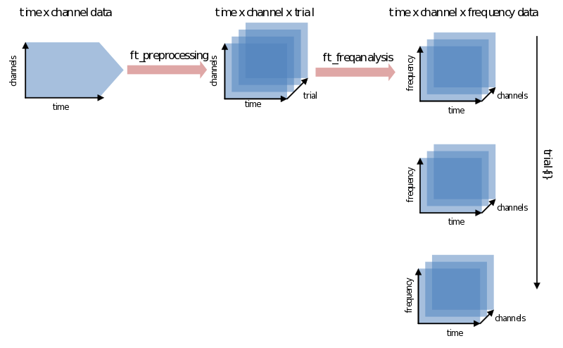
Power per trial

In the simplest case you are interested in the power of certain frequencies (frequencies of interest: cfg.foi) of the whole trial. This is done by using ‘mtmfft’ as the method:

cfg = [];
cfg.method = 'mtmfft';
cfg.output = 'pow';
cfg.foi = [1:30];
cfg.taper = 'dpss';
cfg.tapsmofrq = [2];

Note that in cfg.foi we are now specifying a list of frequencies with steps of 1 Hz. It is also possible to specify a range (cfg.foilim = [1 30];) which will output an average power over these frequencies, or to take different size “steps” (cfg.foi = [1:2:30];).

Power changes over time

The most used method for frequency analysis in FieldTrip besides ‘‘mtmfft’’ is ‘‘mtmconvol’’. There are two main differences between the two. First, ‘‘mtmfft’’ gives the average frequency-content of your trial, whereas ‘‘mtmconvol’’ gives the time-frequency representation of your trial, i.e. how the frequency content of your trial changes over time. Second, they differ in their implementation. Below a short description:

'’Mtmfft’’ consists of 2 main steps.

1. Your raw data is windowed/tapered by a taper you selected in cfg.taper (e.g., hanning, dpss, etc.). This is important for various reasons explained in the next section.
2. the Fast-Fourier-Fransform (FFT) of your data is taken, and parts of this are selected as output.

'’Mtmconvol’’ works a little differently. One of several methods to get a time-frequency representation of your data is by using wavelet-convolution, where a wavelet is ‘sliding’ over your raw data, at each time-point taking the average of a element-wise multiplication of all the data that ‘lies under’ your wavelet. ‘‘Mtmconvol’’ does exactly this, but then by multiplication in the frequency domain (which is much faster than convolution in the time-domain).

1. Wavelets are created, the length determined by ‘‘cfg.tf_timwin’’, with 1 wavelet per frequency.
2. Wavelet is windowed/tapered similarly as step 1 in ‘‘mtmfft’’.
3. The Fast-Fourier-Transform is taken of both your raw data and your wavelet and multiplied with each other (for each frequency).
4. The inverse Fourier-transform is taken, and parts of this are selected as output.

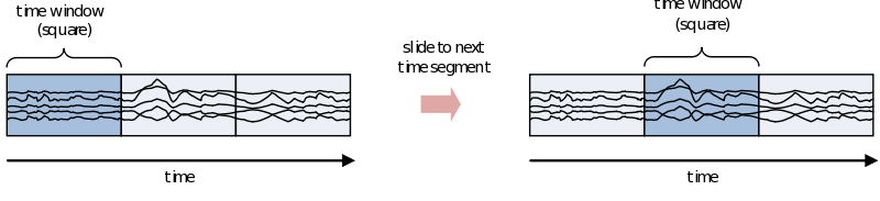
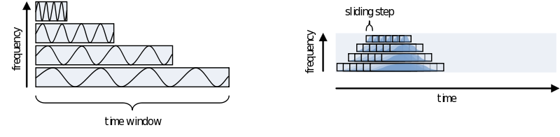
Sliding time windows

If you are interested in the development of the power (or other frequency information beyond the scope of this document) over time, you need to cut up the time course into pieces and calculate the power for every piece separately

However, because of the straight edges of the time window spectral leakage will occur (something you do not want). It is therefore recommended make the edges of the time window taper off to zero by for instance multiplying the time course with an inverted cosine function. This is called a Hanning window:

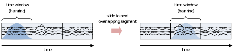
As you can see using such a taper will make you lose data between the time windows. This is compensated by using an overlapping time window, providing the average power of the time-window centered at multiple time-points. Note that although you sample in much smaller steps, the value for every window is still calculated for the whole time window:

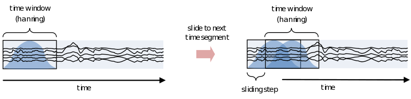
One consideration in choosing the width of your time-window is the wavelength of the frequency you want to calculate. As we view an oscillation as consisting of several cycles, this needs to be reflected in the time-window. Also, you need several cycles captured in your time-window to have a relative reliable estimate of its power during that time. This means that for a signal of 2 Hz the time window should be several times 0.5 seconds (T = 1/f). For higher frequencies this can be much shorter, 30Hz giving you a period of about 33 milliseconds. To not make concessions for one or the other extreme you can make your time-windows dependent on the frequency by making it a multiple of its period. It is recommended to not use less than 3 cycles. Remember, the way you define your window biases your results towards that particular view. If you are searching for long-lasting oscillations and therefore use time-windows of e.g., 10 cycles, your results will reflect that portion of your data most strongly. If, instead, you use a window of 1 cycle, do not expect to see (although you might) oscillations evolving over time, as you are biasing your results against it.

To summarize let’s look at the different parameters that have to be set for doing a frequency analysis with a sliding, frequency dependant, time window, using a Hanning taper and then call ‘‘ft_freqanalysis’’ on one dataset:

cfg.trials         = trialsA;
cfg.output         = 'pow';
cfg.method         = 'mtmconvol';
cfg.taper          = 'hanning';
cfg.foi            = 1:30;
cfg.t_ftimwin      = 4 ./ cfg.foi;
cfg.toi            = -0.5:0.05:2;
freq               = ft_freqanalysis(cfg, data_lp);

Selecting trials using .trialinfo

By default ‘‘ft_freqanalysis’’ (and as we will see, also ‘‘ft_timelockanalysis’’) will not retain information on separate trials but will output the average frequency information (power in this case) over all trials. Also for reasons of memory and speed this might be a good moment to separate your trials into conditions and do a frequency analysis for every condition separately. You can select the trials on which to do ‘‘ft_freqanalysis’’ or ‘‘ft_timelockanalysis’’ by specifying trial indexes in ‘‘cfg.trials’’. The trial index is nothing more than a number pointing to the n-th trial in the data structure. Since we have all the information about the conditions that the trials belong to stored in the ‘‘.trialinfo’’ field, we can search through it to make such a list. Remember we already made a list of trial codes belonging to our two conditions (markersA & markersB). We’ll just search through our ‘‘.trialinfo’’ looking for those trials that match those code

trialsA = [];                                       % make an empty array
for i = 1 : size(markersA,2)                        % start a loop from 1 to the number of items in our markersA array
index = find(data_manual.trialinfo == markersA(i)); % find the index in data_manual.trialinfo that corresponds with the i-th item in the markersA list. If there is not, it will remain empty
trialsA = [trialsA index]                           % add the index to the trialA array
end                                                 % end of loop

We can now add the following line to the cfg:

cfg.trials = trialsA;

However, if you want to save trials separately you can specify the following option:

cfg.keeptrials = 'yes';                             % default = 'no'

Output of ft_freqanalysis

We might go further into the output of ft_freqanalysis in a future release of this document but for now it suffices to say it gives a datastructure as output similar as the input structure but now with the field ‘‘.powspctrm’’ instead of ‘‘.trial’’ or ‘‘.avg.trial’’. For further information see timefrequencyanalysis and plotting.

Statistics

FieldTrip distinguishes itself perhaps most in its flexibility in statistical approaches. In a similar way as with ft_definetrial and ft_freqanalysis, ft_timelockedstatistics and ft_freqstatistics call auxiliary functions to calculate the different statistics. Don’t be afraid though – most users won’t need to go nitty-gritty and go through those functions. As an end user needs to understand most of all it:

1. The difference between descriptive and inferential statistics
2. The common structure for the input to - and output from - ft_freqstatistics

Descriptive & inferential statistic

The difference between descriptive and inferential statistic is often implicit in neuroimaging analysis packages, or in research articles for that matter. It really pays off to consider them separately here and to entertain the many possibilities of combining descriptive statistics with statistical methods. It is paramount in understanding the philosophy and appreciating the full statistical potential of FieldTrip.

So what do we mean with descriptive statistic? It’s the single value you end up with after reducing your data(set) and representing an aspect of its distribution which you would want to use for statistical comparison. Think for instance about “average alpha power over trials”, “variance of the P300 amplitude” or “the latency of maximal mu-rhythm suppression”. You might calculate a descriptive statistic for every subject, e.g., the difference between conditions (which you want to compare over subjects). Conversely, you might want to use one descriptive for every trial (which you will compare within a subject). A descriptive statistic is not limited to averages of power or amplitude but can be any output of a statistical procedure itself, such as a Z-value, t-value, variance, mean-difference or Beta-value. The inferential statistic is what you get when you test your descriptive statistics against the null-hypothesis, e.g., is your p-value. Again, there are many ways to do your null-hypothesis testing, e.g., using a (paired) t-test or Monte Carlo approach.

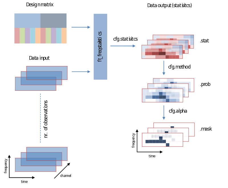
Input – output structure of ft_freqstatistics

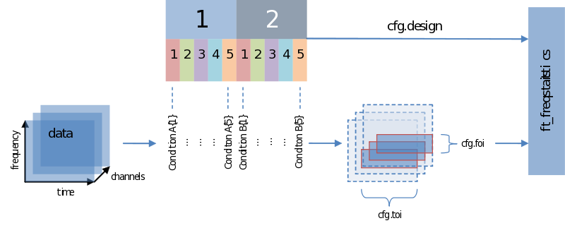
Also when it comes to your statistical analysis FieldTrip doesn’t let you down: The structure of its output is consistent with the data structure of its input. We will revisit the following figure a couple of times, but for now please notice:

1. Unless you specify otherwise through averaging on a certain dimension, the structure of the output will have the same structure as the input
2. Those values of the output – the descriptive statistics, the inferential statistics and the decisions (to reject your null-hypothesis), are dependent on cfg.statistic, cfg.method and cfg.alpha, respectively.
3. That we need to specify a design matrix – our next topic

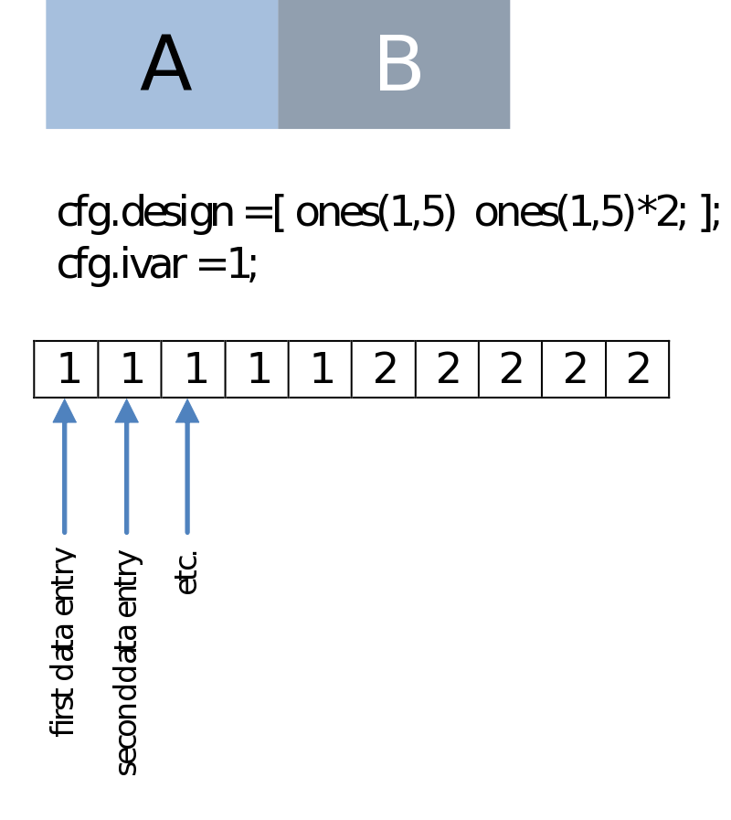
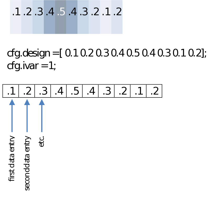
Input - data and your design matrix

It should be obvious that besides feeding data we need to specify how the separate data entries should be treated – which belong to the same condition for instance. What is common to all designs is that data entries are always assumed to be in a row. In the simplest case we only need to specify a code corresponding to the independent variable for every data entry. Note the use of the parameters ivar and uvar. They denote nothing more than the row-number in the design-matrix to find either your independent variables (ivar) or units of observation (uvar).

Non-paired comparison

This could be simply the condition number as we have in the case of a (non-paired) comparison of two series of data entries. Note that this is the same regardless if we are dealing with a within-subject (e.g., condition A versus B) or a between-subject design (e.g., group A versus B, session A versus B):

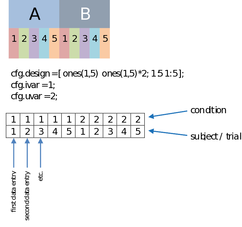
Paired comparison

Besides a row coding for the independent variable such as your experimental condition (the first row, therefore: cfg.ivar = 1;), we can code for every dependant variable, or unit of observation in the second row (uvar = 2); The units of observation often are subjects (in a certain group) or trials (of a certain condition), for instance. This allows us to do a paired comparison. The example below is just an example, there is no necessity to have such an organized design, as long as you make sure every n-th column corresponds to the appropriate n-th data entry.

Correlation

You might not want to test groups but rather calculate a correlation with any other series of values. These could be reaction times, a subject score on a questionnaire or even power in another frequency. Your design then will only have to specify those in a single row. For the example below we’ll just make an imaginary [sic] array of values.

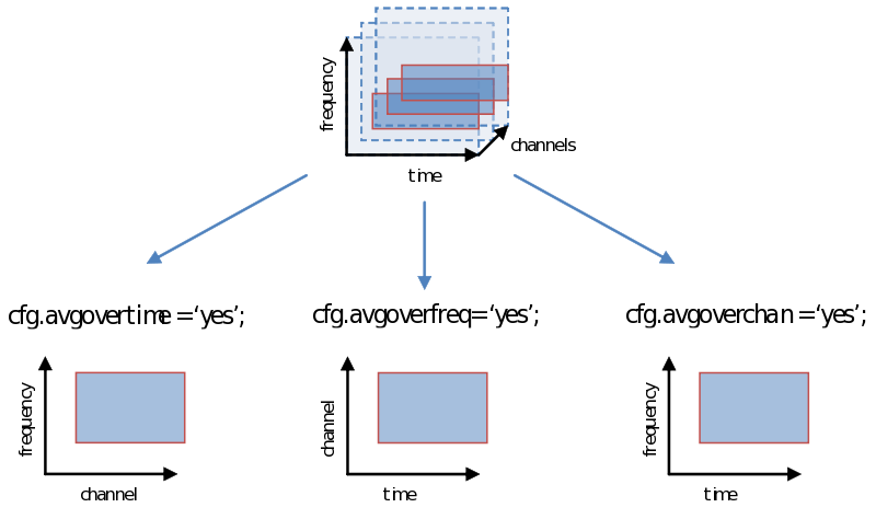
Averaging over time/frequencies/sensors

As you are well aware, however, the decision we make using the statistical test (not to be confused with the test-statistic) is vulnerable to the multiple comparison problem, a problem that is greatly exacerbated with the multidimensional nature of psychophysiological data. One way of dealing with this problem is simply to average over (parts of) a dimension. Doing this now, instead of earlier during ft_preprocessing, ft_freqanalysis or ft_timelockanalysis gives us all the flexibility to explore different windows on which to calculate our test statistic (“average power of…”, or “average amplitude of…”). Remember how we showed in the previous page to specify a time-frequency window or select channels. We can simply average over one of these dimensions as follows:

Statistical methods

Once the design matrix is specified and the test statistic is defined we only need to decide how we are going to test our hypothesis. Of course the statistical methods one will use are somewhat dependent on the design matrix you specified but let’s just summarize them all here:

• ft_statistics_analytic
• ft_statistics_crossvalidate
• ft_statistics_montecarlo
• ft_statistics_stats

Calling ft_freqanalysis