workshop / baci2017 / forwardproblem /
Solving the EEG forward problem using BEM and FEM
Introduction
The aim of this tutorial is to solve the EEG forward problem using two different numerical methods, namely the Boundary Element Method (BEM) and the Finite Element Method (FEM).
Background
The EEG/MEG signals measured on or around the scalp do not directly reflect the activated neurons in the brain. To reconstruct the actual activity in the brain, source reconstruction techniques are used. You can read more about the different methods in the review papers that are listed here.
The activity in the brain is estimated from the EEG or MEG signals using
- the EEG/MEG activity itself that is measured on or around the scalp
- the spatial arrangement of the electrodes/gradiometers relative to the brain (sensor positions),
- the geometrical and conductive properties of the head (head model)
- the location of the source (source model)
Using this information, source estimation comprises two major steps: (1) Estimation of the EEG potential or MEG field distribution for a known source is referred to as forward modeling. (2) Estimation of the unknown sources corresponding to the measured EEG or MEG is referred to as inverse modeling.
The forward solution can be computed when the head model, the sensor positions and a model for the source are given. For distributed source models and for scanning approaches such as beamforming, the source model consists of a discrete description of the brain volume or of the cortical sheet in many voxels or vertices. When the forward solution is computed, the lead field matrix (with dimensions Nchan * Nsources) is calculated for each point, taking into account the head model and the sensor positions.
A prerequisite of forward modeling is that the geometrical description of the sensor positions, head model and source model are expressed in the same coordinate system (e.g., CTF, MNI, Talairach) and with the same units (mm, cm, or m). There are different conventions for coordinate systems. The precise coordinate system is not relevant, as long as all data is consistent. Here you can read how the different head and MRI coordinate systems are defined. For most MEG systems, the gradiometers are by default defined relative to head localizer coils or anatomical landmarks, therefore when the anatomical MRI are aligned to the same landmarks, the position of the MEG sensors directly matches the MRI. As EEG data is typically not explicitly aligned relatively to the head, therefore, the EEG electrodes usually have to be explicitly realigned prior to source reconstruction (see also this faq and this example).
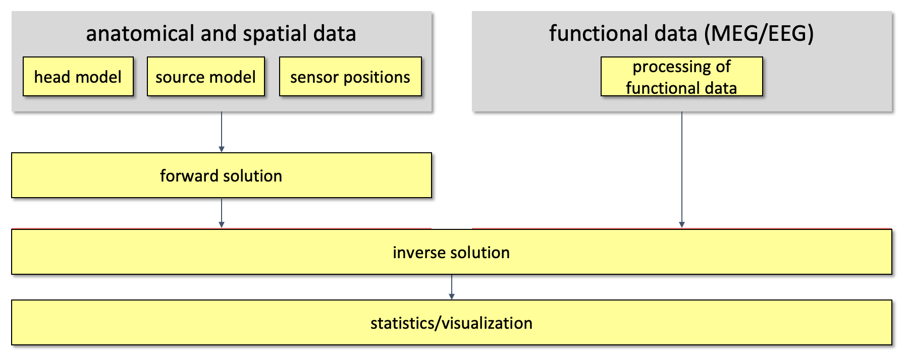
Figure 1. Overall outline of the pipeline used for source reconstruction
Procedure
As already mentioned, the goal of this session is to solve the EEG forward problem, more precisely we want to compute EEG leadfields so that the inverse problem can be solved in the next session (inverse problem).
To compute the leadfields, there are 9 main steps that have to be followed.
- Load and read the anatomical data, namely a T1-MRI (ft_read_mri);
- Align the MRI to the electrodes. As the electrodes are expressed in the CTF coordinate system, we translate the MRI in the CTF coordinate system (ft_volumerealign);
- Reslice the MRI image so that the voxels of the anatonical data are homogeneous (i.e. the size of the voxel is the same into each direction). This step will facilitate the segmentation step. (ft_volumereslice)
- Segment the MRI: 3 compartments for BEM (scalp, skull, brain) and 5 compartments for FEM (scalp, skull, CSF, grey matter and white matter) (ft_volumesegment);
- then we create the mesh: triangulated surface mesh for BEM and hexahedral volume mesh for FEM (ft_prepare_mesh).
- Create the headmodels (headmodel_bem and headmodel_fem) where geometrical and electrical information are merged together (ft_prepare_headmodel);
- Align the electrodes to the MRI (ft_electroderealign);
- The sourcemodel is created, where the location of the sources is restrained to the brain compartment (from the BEM mesh) (ft_prepare_sourcemodel);
- Leadfields can be computed (ft_prepare_leadfield).
The first 3 steps are the same for BEM and FEM. Steps from 4 to 8 differ between BEM and FEM. A more detailed description of these steps is following.
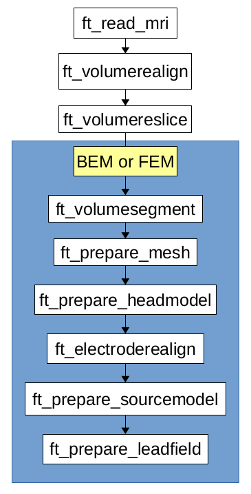
Figure 1: pipeline for forward computation, in the blue box there are the steps which differ between BEM and FEM
1. Read the MRI
mri_orig = ft_read_mri('subject01.nii');
Visualize the MRI.
cfg = [];
ft_sourceplot(cfg, mri_orig);
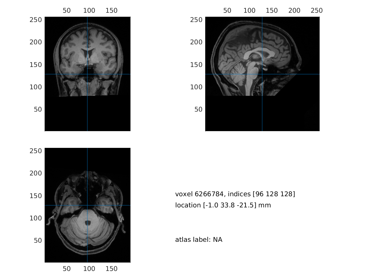
Figure 2: visualization of the MRI
2. Realign the MRI
In this step we will interactively align the MRI to the CTF space. We will be asked to identify the three CTF landmarks (nasion, NAS; right pre-auricular point, RPA; left pre-auricular point, LPA) in the MRI.
cfg = [];
cfg.method = 'interactive';
cfg.coordsys = 'ctf';
mri_realigned = ft_volumerealign(cfg, mri_orig);
We can visualize the realigned MRI
cfg = [];
ft_sourceplot(cfg, mri_realigned);
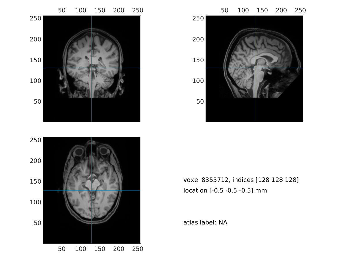
Figure 3: visualization of the realigned MRI
3. Reslice the MRI
cfg = [];
mri_resliced = ft_volumereslice(cfg, mri_realigned);
We can visualize the resliced MRI
cfg = [];
ft_sourceplot(cfg, mri_resliced);
A. Boundary Element Method (BEM)
4A. Segment the MRI
cfg = [];
cfg.output = {'brain', 'skull', 'scalp'};
mri_segmented_3_compartment = ft_volumesegment(cfg, mri_resliced);
Visualize the segmentation
seg_i = ft_datatype_segmentation(mri_segmented_3_compartment, 'segmentationstyle', 'indexed');

cfg = [];
cfg.funparameter = 'seg';
cfg.funcolormap  = gray(4); % distinct color per tissue
cfg.location     = 'center';
cfg.atlas        = seg_i;
ft_sourceplot(cfg, seg_i);
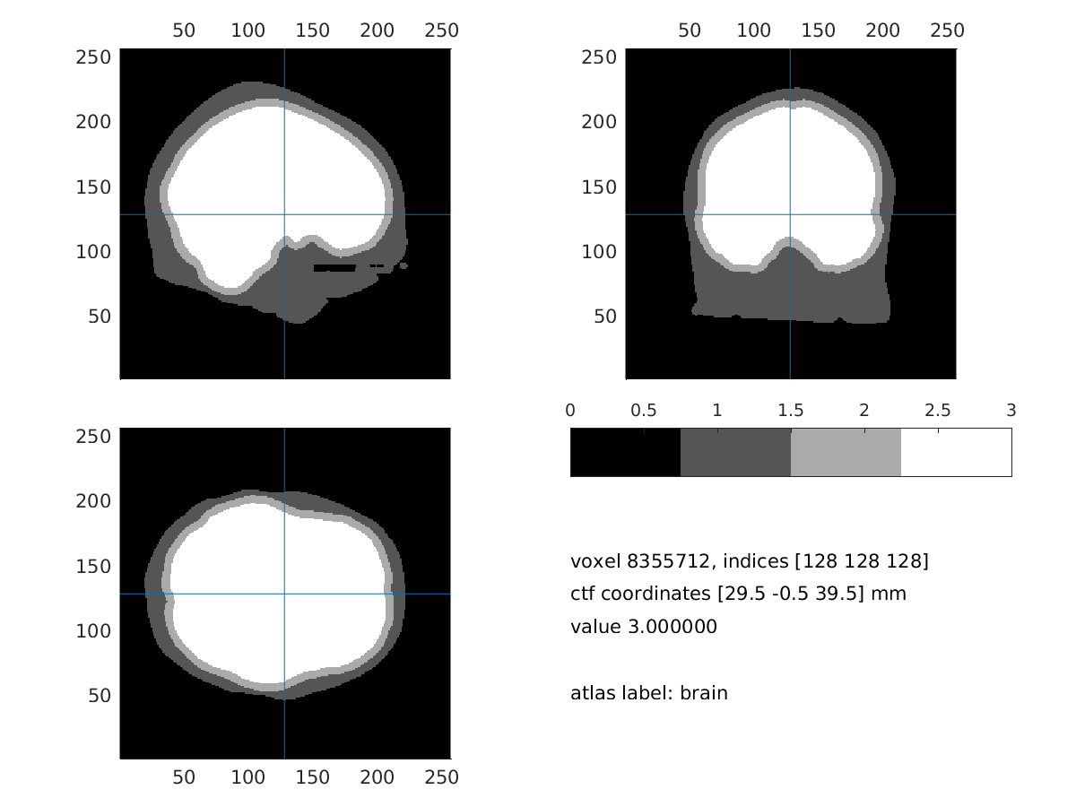
Figure 4: 3 compartment segmentation output
5A. Create the mesh
cfg = [];
cfg.tissue = {'brain', 'skull', 'scalp'};
cfg.numvertices = [3000 2000 1000];
mesh_bem = ft_prepare_mesh(cfg, mri_segmented_3_compartment);
Visualize the mesh and the electrode
load elec; %load the electrodes
figure, ft_plot_mesh(mesh_bem(1), 'surfaceonly', 'yes', 'vertexcolor', 'none', 'facecolor', 'skin', 'facealpha',0.5, 'edgealpha',0.1)
ft_plot_mesh(mesh_bem(2), 'surfaceonly', 'yes', 'vertexcolor', 'none', 'facecolor', 'skin', 'facealpha',0.5, 'edgealpha',0.1)
ft_plot_mesh(mesh_bem(3), 'surfaceonly', 'yes', 'vertexcolor', 'none', 'facecolor', 'skin', 'facealpha',0.5, 'edgealpha',0.1)
hold on, ft_plot_sens(elec, 'style', '*g');
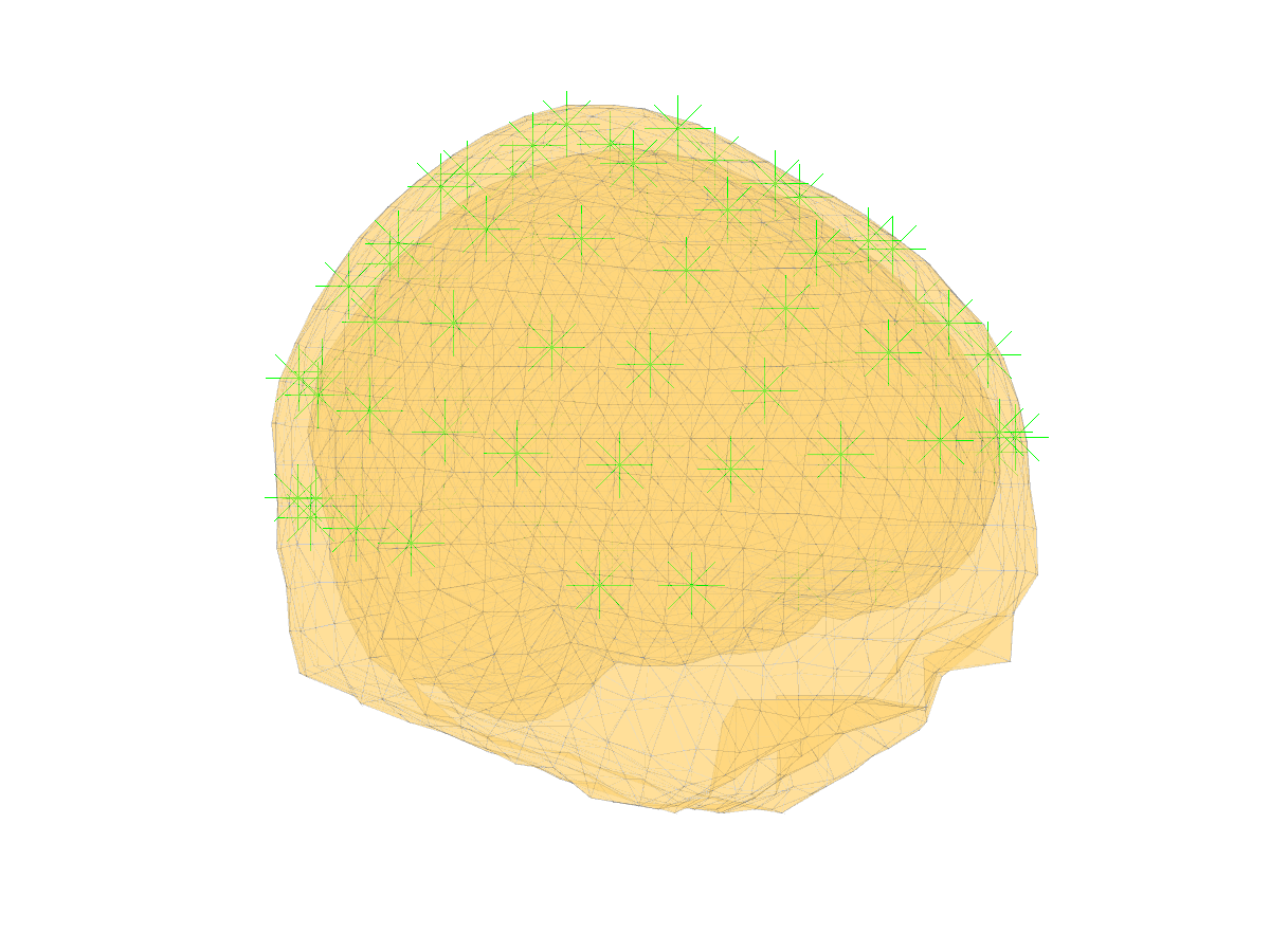
Figure 5: 3 compartment mesh with electrodes
6A. Create the headmodel
cfg = [];
cfg.method ='dipoli'; % You can also specify 'bemcp', or another method.
headmodel_bem       = ft_prepare_headmodel(cfg, mesh_bem);
In Windows the method ‘dipoli’ does not work. You can either load “headmodel_bem” and continue with this tutorial, or explore other BEM method like ‘bemcp’. If you use ‘bemcp’, the conductivity field has a different order: {‘brain’, ‘skull’, ‘skin’}.
7A. Align the electrodes
If the electrodes are not well aligned with the mesh, we can realign them with:
cfg = [];
cfg.method    = 'interactive';
cfg.elec      = elec;
cfg.headshape = headmodel_bem.bnd;
elec = ft_electroderealign(cfg);
Check the alignment visually.
figure;
ft_plot_axes(mesh_bem)
hold on;
ft_plot_mesh(mesh_bem.bnd(1), 'surfaceonly', 'yes', 'vertexcolor', 'none', 'facecolor', 'skin', 'facealpha',0.5, 'edgealpha',0.1)
ft_plot_sens(elec, 'style', '.k');
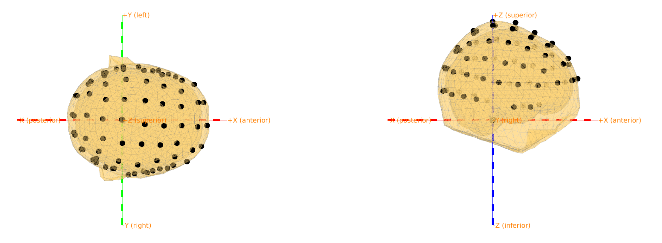
Figure 6: mesh, electrodes and axes.
8A. Create the sourcemodel
cfg = [];
cfg.resolution  = 7.5;
cfg.threshold   = 0.1;
cfg.smooth      = 5;
cfg.headmodel   = headmodel_bem;
cfg.inwardshift = 1; % shifts dipoles away from surfaces
sourcemodel = ft_prepare_sourcemodel(cfg);
Visualize the sourcemodel
figure, ft_plot_mesh(sourcemodel.pos(sourcemodel.inside,:))
hold on, ft_plot_mesh(mesh_bem.bnd(1), 'surfaceonly', 'yes', 'vertexcolor', 'none', 'facecolor',...
           'skin', 'facealpha',0.5, 'edgealpha',0.1)
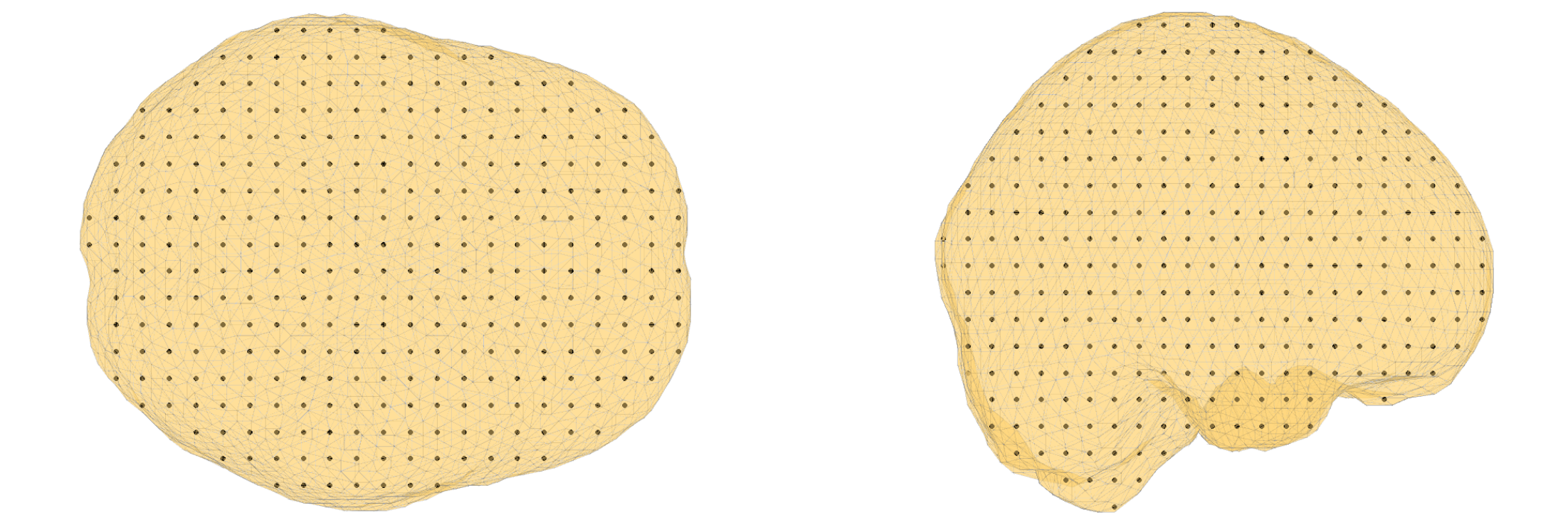
Figure 7: sourcemodel on the brain compartment
Save the sourcemode
save sourcemodel sourcemodel;
9A. Compute the leadfield
cfg = [];
cfg.grid        = sourcemodel;
cfg.headmodel   = headmodel_bem;
cfg.elec        = elec;
cfg.reducerank  = 3;
leadfield_bem = ft_prepare_leadfield(cfg);
B. Finite Element Method (FEM)
4B. Segment the MRI
cfg = [];
cfg.output         = {'scalp', 'skull', 'csf', 'gray', 'white'};
cfg.brainsmooth    = 1;
cfg.scalpthreshold = 0.11;
cfg.skullthreshold = 0.15;
cfg.brainthreshold = 0.15;
mri_segmented_5_compartment = ft_volumesegment(cfg, mri_resliced);
Visualize the segmentation result
seg_i = ft_datatype_segmentation(mri_segmented_5_compartment, 'segmentationstyle', 'indexed');

cfg = [];
cfg.funparameter = 'seg';
cfg.funcolormap  = gray(5); % distinct color per tissue
cfg.location     = 'center';
cfg.atlas        = seg_i;    % the segmentation can also be used as atlas
ft_sourceplot(cfg, seg_i);
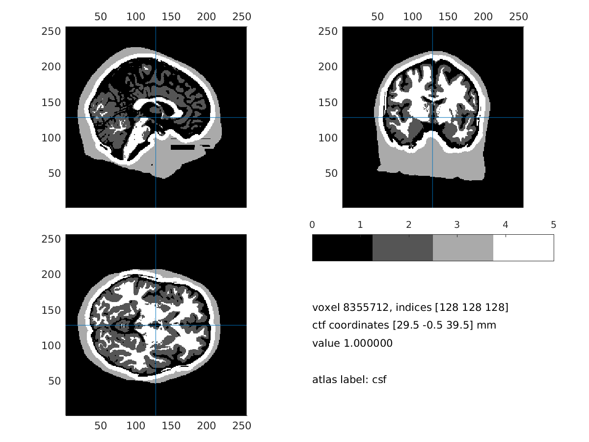
Figure 8: 5 compartment segmentation output
5B. Create the mesh
cfg = [];
cfg.shift  = 0.3;
cfg.method = 'hexahedral';
cfg.resolution = 1; % this is in mm
mesh_fem = ft_prepare_mesh(cfg,mri_segmented_5_compartment);
6B. Create the headmodel
cfg = [];
cfg.method = 'simbio';
cfg.conductivity = [0.43 0.0024 1.79 0.14 0.33]; % same as tissuelabel in vol_simbio
cfg.tissuelabel = {'scalp', 'skull', 'csf', 'gray', 'white'};
headmodel_fem = ft_prepare_headmodel(cfg, mesh_fem);
Visualize the headmodel and the electrodes (it might take time and memory)
% csf: 1, gm: 2, scalp: 3, skull: 4, wm: 5
ts = 3;
figure
mesh2 =[];
mesh2.hex = headmodel_fem.hex(headmodel_fem.tissue==ts,:); %mesh2.hex(1:size(mesh2.hex),:);
mesh2.pos = headmodel_fem.pos;
mesh2.tissue = headmodel_fem.tissue(headmodel_fem.tissue==ts,:); %mesh.tissue(1:size(mesh2.hex),:);

mesh_ed = mesh2edge(mesh2);
patch('Faces',mesh_ed.poly,...
  'Vertices',mesh_ed.pos,...
  'FaceAlpha',.5,...
  'LineStyle', 'none',...
  'FaceColor',[1 1 1],...
  'FaceLighting', 'gouraud');

xlabel('coronal');
ylabel('sagital');
zlabel('axial')
camlight;
axis on;

ft_plot_sens(elec, 'style', '*g');
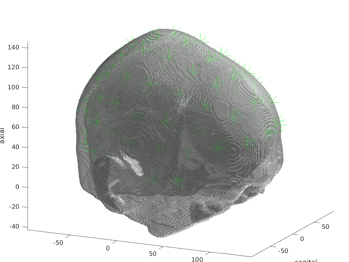
Figure 9: visualization of headmodel_fem and electrodes
7B. Align the electrodes
If the electrodes are not well aligned with the mesh, we can realign them with:
cfg           = [];
cfg.method    = 'interactive';
cfg.elec      = elec;
cfg.headshape = headmodel_fem;
elec = ft_electroderealign(cfg);
8B. Create the sourcemodel
We will use the sourcemodel already generated in 7A.
load('sourcemodel.mat');
9B. Compute the leadfield
Please DO NOT run ft_prepare_vol_sens in this tutorial session! It will take too much time and memory. Load headmodel_fem_tr.mat from disk instead.
% compute the transfer matrix
[headmodel_fem_tr, elec] = ft_prepare_vol_sens(headmodel_fem, elec);

% compute the leadfield
cfg = [];
cfg.grid = sourcemodel;
cfg.headmodel= headmodel_fem_tr;
cfg.elec = elec;
cfg.reducerank = 3;
leadfield_fem = ft_prepare_leadfield(cfg);
Summary and Comments
This tutorial was about the computation of leadfields that could be feed into the inverse problem which will be explain in the part on the inverse problem.
This tutorial was last tested on 27-08-2017 by Maria Carla Piastra on Ubuntu, Matlab 2015b.