workshop / baci2017 / inverseproblem /
Solving the EEG inverse problem
Introduction
In this tutorial you can find information about how to fit dipole models and how to do source reconstruction using minimum-norm estimation to the somatosensory evoked potentials (SEPs) of a single subject from the preprocessing.
We will be working on the dataset from the previous hands on sessions, and we will use the functional and anatomical data from these tutorials to deal with the inverse problem. As you already noticed we have prepared two different mathematical models from the forward problem. We will use both to solve the inverse problem and compare the results. You’ve either got the relevant data already processed yourself or can find in the data directory.
This tutorial will not show how to combine source-level data over multiple subjects. It will also not describe how to do source-localization of oscillatory activation. You can check the Localizing oscillatory sources using beamformer techniques tutorial if you are interested in the later.
Background
Dipole fit
In this tutorial we will use the dipole fitting approach (1) to localise the neuronal activity and (2) to estimate the time course of the activity. This approach is most suitable for relatively early cortical activity which is not spread over many or large cortical areas. Dipole fitting assumes that a small number of point-like equivalent current dipoles (ECDs) can describe the measured topography. It optimises the location, the orientation and the amplitude of the model dipoles in order to minimise the difference between the model and measured topography. A good introduction to dipole fitting is provided by Scherg (Source localization by fitting an equivalent current dipole model Scherg M. Fundamentals of dipole source potential analysis. In: Auditory evoked magnetic fields and electric potentials. eds. F. Grandori, M. Hoke and G.L. Romani. Advances in Audiology, vol. 6. Karger, Basel, pp 40-69, 1990).
Minimum norm estimate
To calculate distributed neuronal activation we will use the minimum-norm estimation. This approach is favored for analyzing evoked responses and for tracking the wide-spread activation over time. It is a distributed inverse solution that discretizes the source space into locations on the cortical surface or in the brain volume using a large number of equivalent current dipoles. It estimates the amplitude of all modeled source locations simultaneously and recovers a source distribution with minimum overall energy that produces data consistent with the measurement (Ou, W., Hämäläinen, M., Golland, P., 2008, A Distributed Spatio-temporal EEG/MEG Inverse Solver. Jensen, O., Hesse, C., 2010, Estimating distributed representation of evoked responses and oscillatory brain activity, In: MEG: An Introduction to Methods, ed. by Hansen, P., Kringelbach, M., Salmelin, R., doi:10.1093/acprof:oso/9780195307238.001.0001). The reference for the implemented method is Dale et al. (2000).
BEM
Dipole fit
First we load the relevant data
load elec
load sourcemodel
load headmodel_bem
load leadfield_bem
load mri_resliced
load EEG_avg
Then we do the dipole fit
% Dipole fit
cfg = [];
cfg.numdipoles    = 1;                              % number of expected
cfg.headmodel     = headmodel_bem;                  % the head model
cfg.grid          = leadfield_bem;                  % the precomputed leadfield
cfg.elec          = elec;                           % the electrode model
cfg.latency       = 0.025;                          % the latency of interest
dipfit_bem        = ft_dipolefitting(cfg,EEG_avg);

disp(dipfit_bem.dip)
ans =
   pos: [13.958237048680118 34.388465910583285 97.809684095994314] % dipole position
   mom: [3x1 double]                                               % dipole moment
   pot: [74x1 double]                                              % potential at the electrodes
    rv: 0.034549469532012                                          % residual variance
  unit: 'mm'
A quick look at dipfit_bem.dip gives us information about the dipole fit. Especially a low residual variance (rv) shows us that the fitted dipole quite well explains the data.
And we visualize the dipole and see where it was localized in the brain.
ft_plot_mesh(headmodel_bem.bnd(3));
alpha 0.7;
ft_plot_dipole(dipfit_bem.dip.pos(1,:), mean(dipfit_bem.dip.mom(1:3,:),2), 'color', 'b','unit','mm')
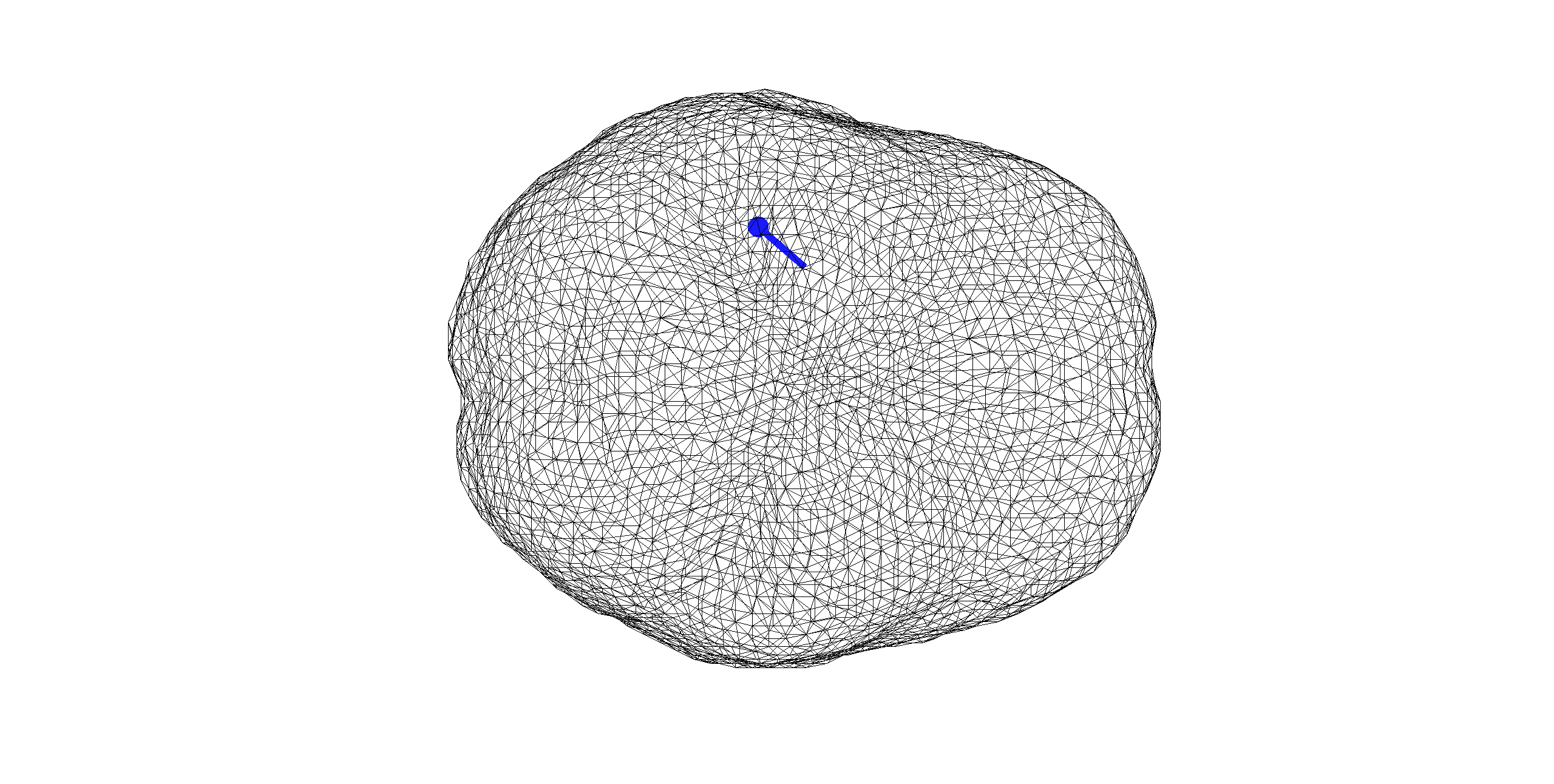
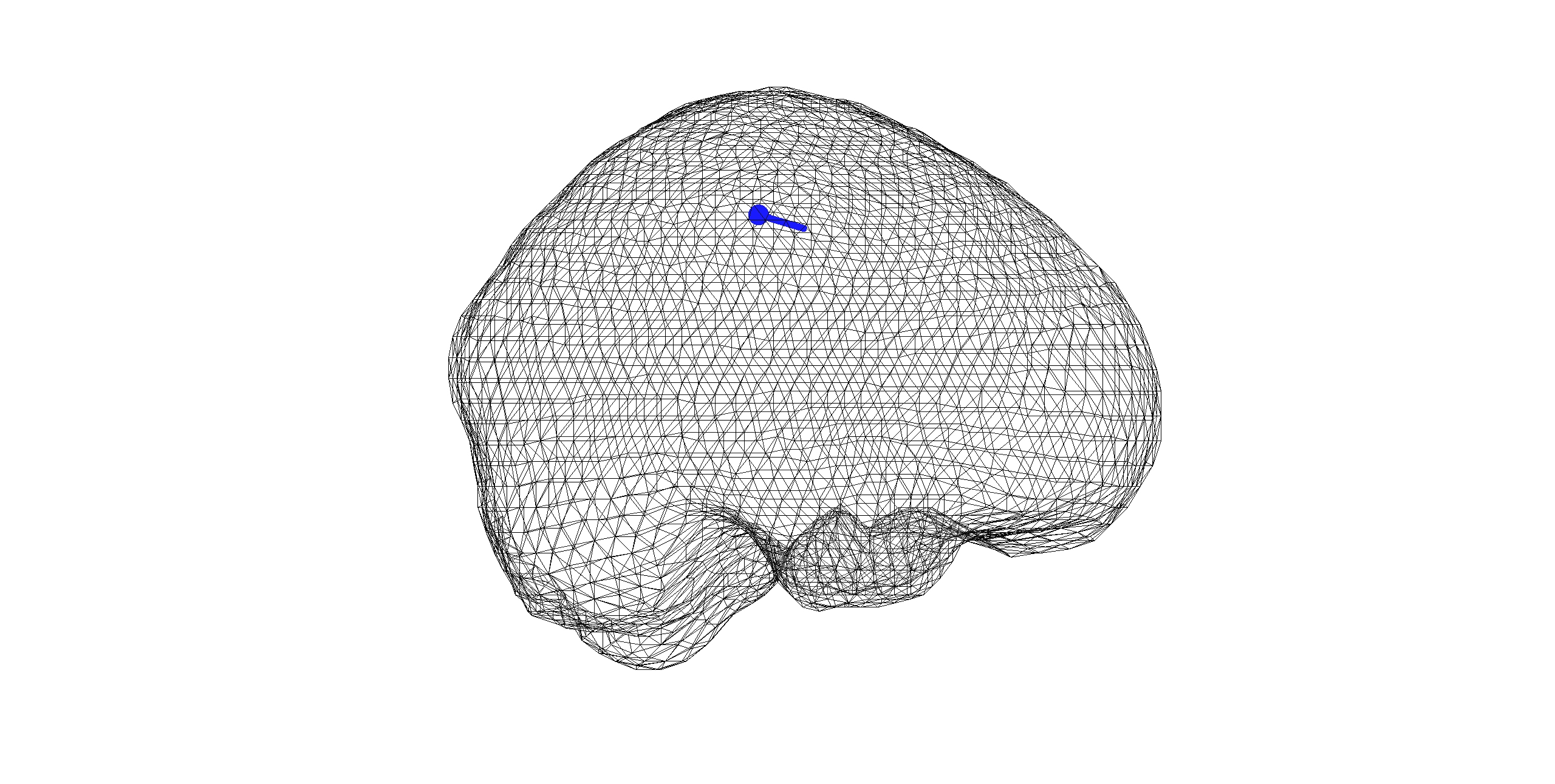
Figure 1. Dipole computed with BEM model
Minimum norm estimate
cfg                     = [];
cfg.method              = 'mne';                    % specify minimum norm estimate as method
cfg.latency             = [0.024 0.026];            % latency of interest
cfg.grid                = leadfield_bem;            % the precomputed leadfield
cfg.headmodel           = headmodel_bem;            % the head model
cfg.mne.prewhiten       = 'yes';                    % prewhiten data
cfg.mne.lambda          = 3;                        % regularisation parameter
cfg.mne.scalesourcecov  = 'yes';                    % scaling the source covariance matrix
minimum_norm_bem        = ft_sourceanalysis(cfg, EEG_avg);
For the purpose of visualization we internet the MNE results onto the replaced anatomical MRI.
cfg            = [];
cfg.parameter  = 'avg.pow';
interpolate    = ft_sourceinterpolate(cfg, minimum_norm_bem , mri_resliced);

cfg = [];
cfg.method        = 'ortho';
cfg.funparameter  = 'pow';
ft_sourceplot(cfg, interpolate);
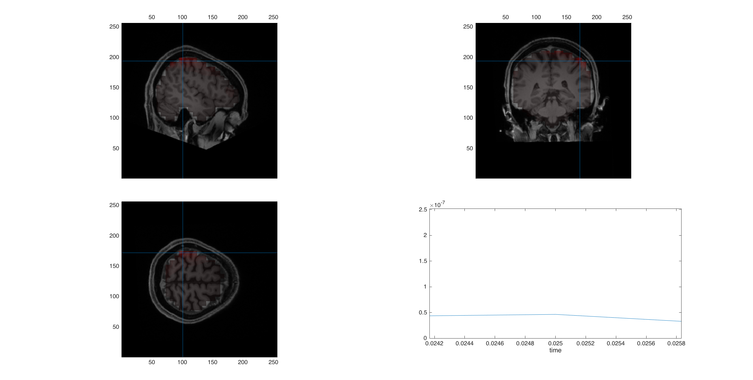
Figure 2. Minimum norm estimation with BEM model
Exercise 1
You can play around with cfg.mne.lambda? Do you see the influence of different lambdas?
FEM
%% FEM
load elec
load sourcemodel
load headmodel_fem_tr
load leadfield_fem
load mri_resliced
load EEG_avg

%% dipole fit
cfg = [];
cfg.numdipoles    = 1;
cfg.grid          = sourcemodel;
cfg.headmodel     = headmodel_fem_tr;
cfg.grid          = leadfield_fem;
cfg.elec          = elec;
cfg.latency       = 0.025;
dipfit_fem        = ft_dipolefitting(cfg,EEG_avg);

ft_plot_mesh(headmodel_bem.bnd(3));alpha 0.7;
ft_plot_dipole(dipfit_fem.dip.pos(1,:), mean(dipfit_fem.dip.mom(1:3,:),2), 'color', 'r','unit','mm')
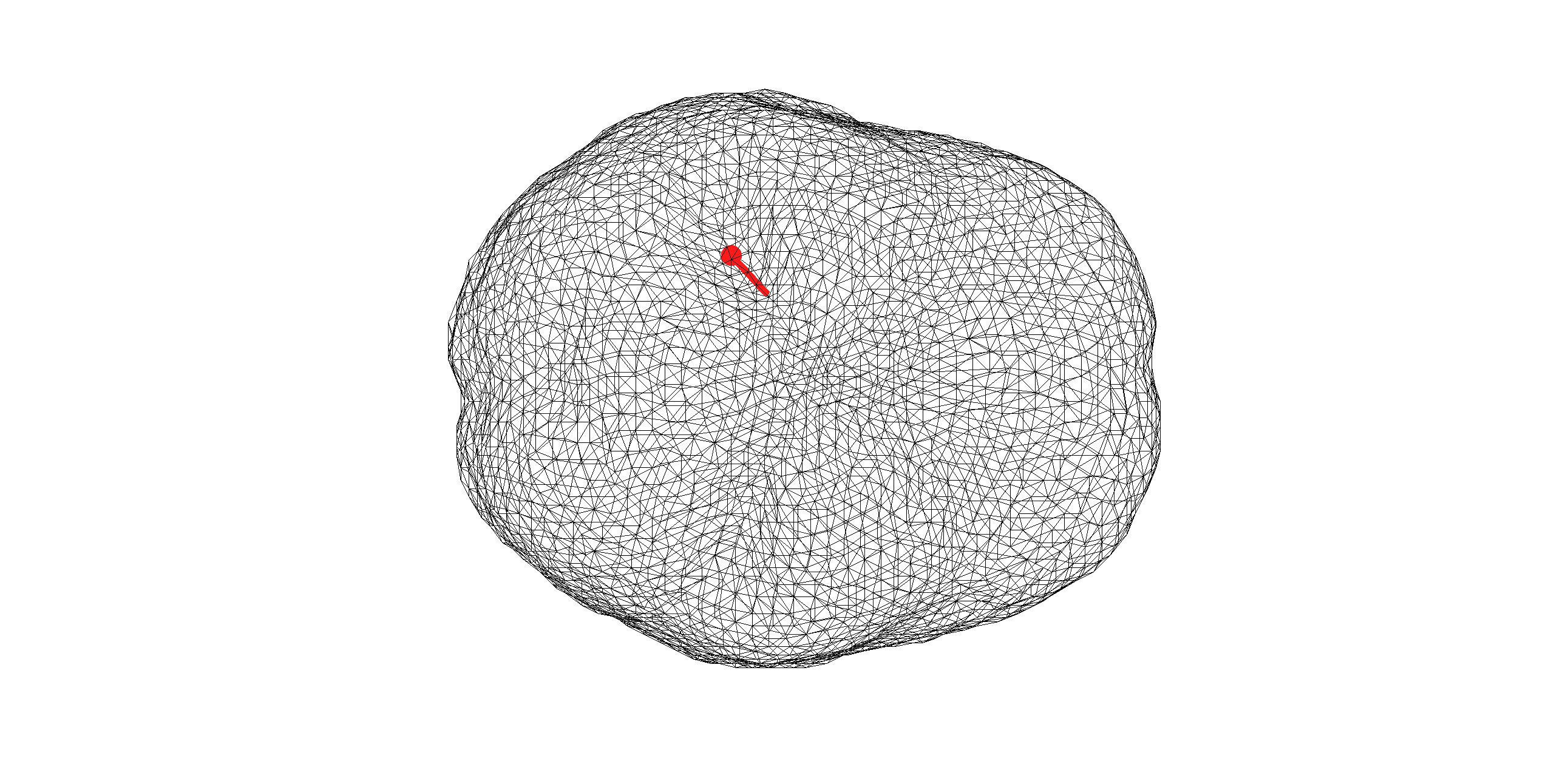
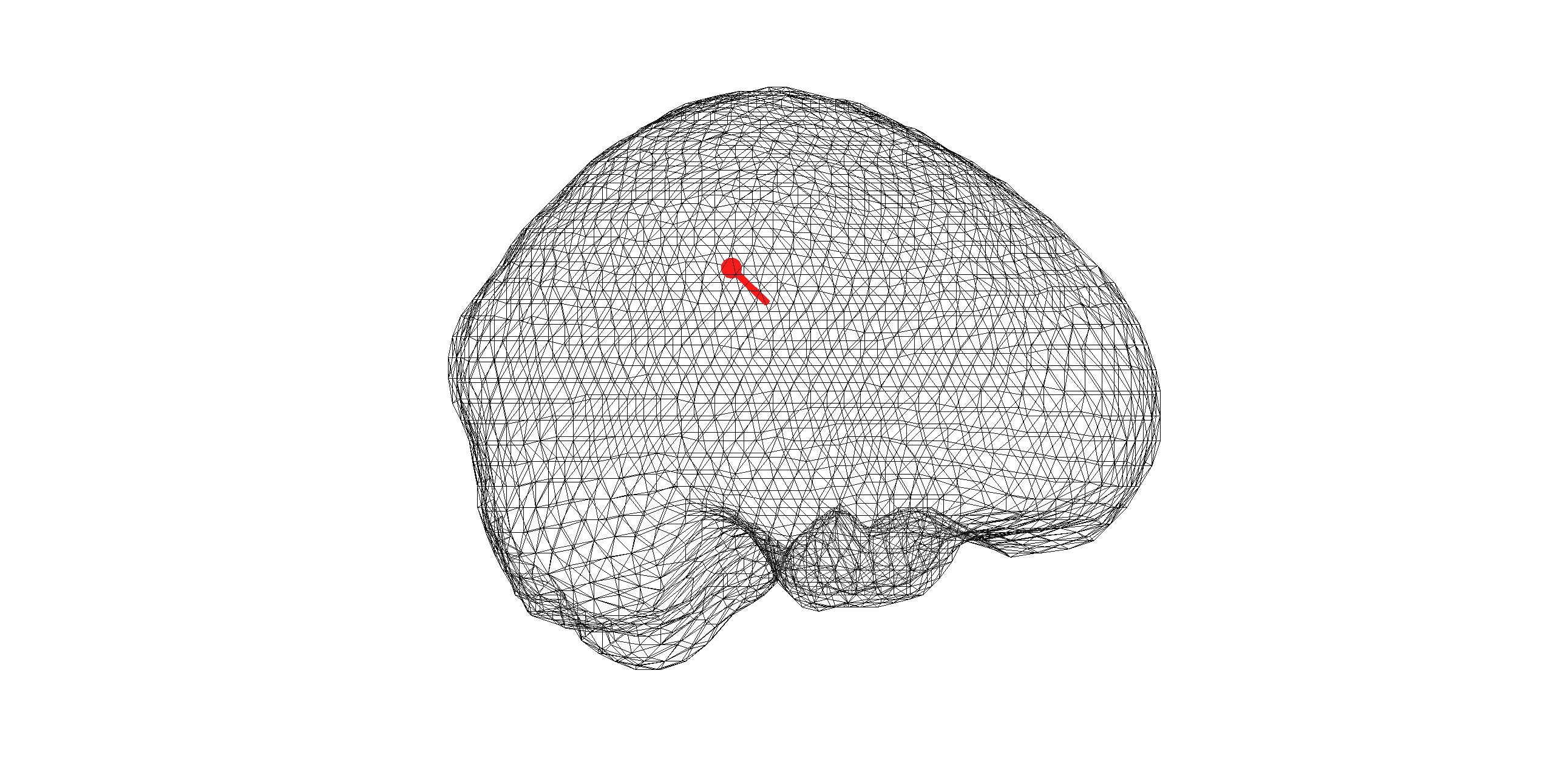
Figure 3. Dipole computed with FEM model
% Minimum norm estimate
cfg = [];
cfg.method        = 'mne';
cfg.latency       = [0.024 0.026];
cfg.grid          = leadfield_fem;
cfg.headmodel     = headmodel_fem_tr;
cfg.mne.prewhiten = 'yes';
cfg.mne.lambda    = 3;
cfg.mne.scalesourcecov = 'yes';
minimum_norm  = ft_sourceanalysis(cfg, EEG_avg);

cfg = [];
cfg.parameter = 'avg.pow';
interpolate = ft_sourceinterpolate(cfg, minimum_norm , mri_resliced);

cfg = [];
cfg.funparameter  = 'pow';
cfg.method        = 'ortho';
ft_sourceplot(cfg, interpolate);
Figure 4. Minimum norm estimation with FEM model
Comparison of BEM and FEM
ft_plot_mesh(headmodel_bem.bnd(3));alpha 0.7;
ft_plot_dipole(dipfit_fem.dip.pos(1,:), mean(dipfit_fem.dip.mom(1:3,:),2), 'color', 'r','unit','mm')
ft_plot_dipole(dipfit_bem.dip.pos(1,:), mean(dipfit_bem.dip.mom(1:3,:),2), 'color', 'b','unit','mm')
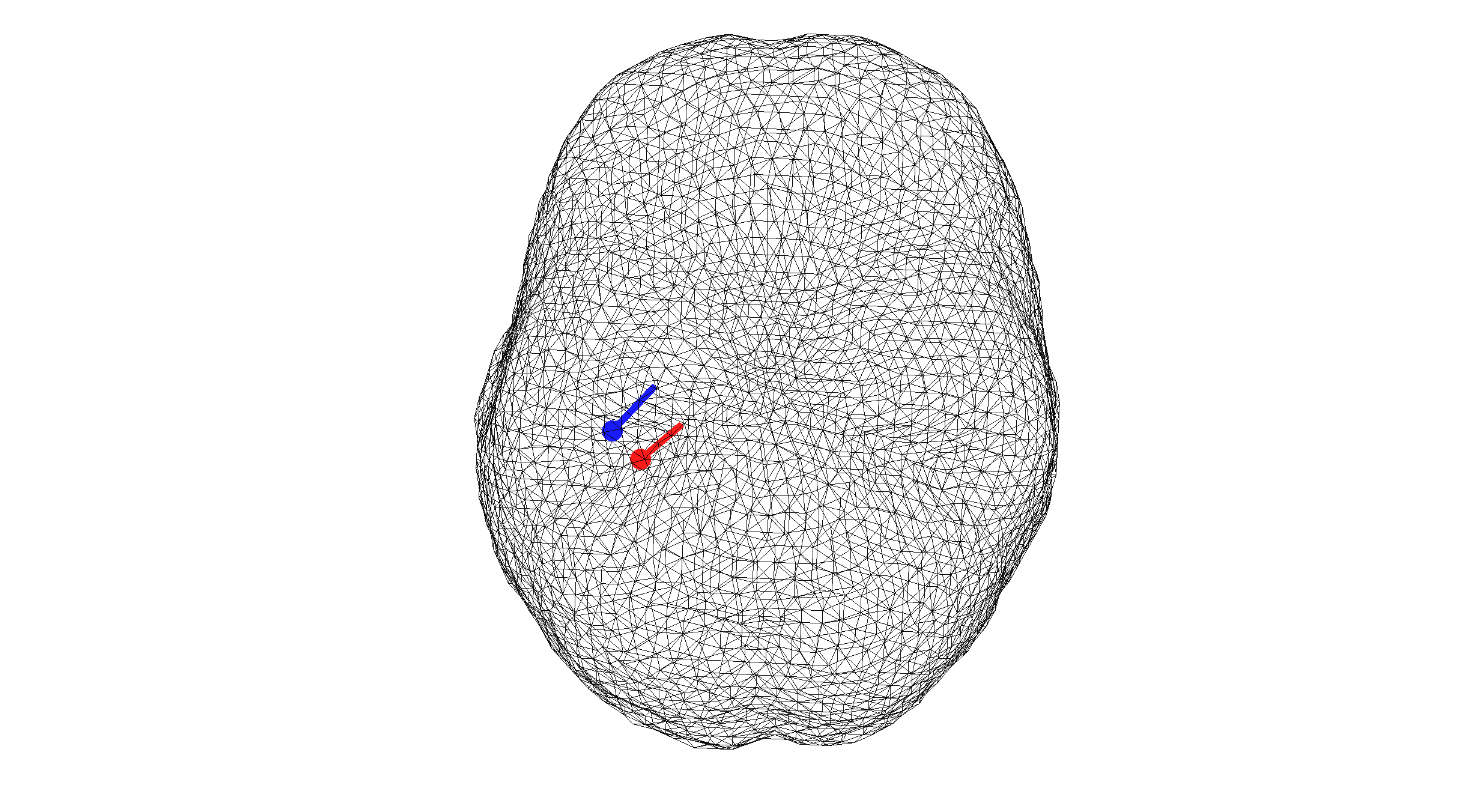
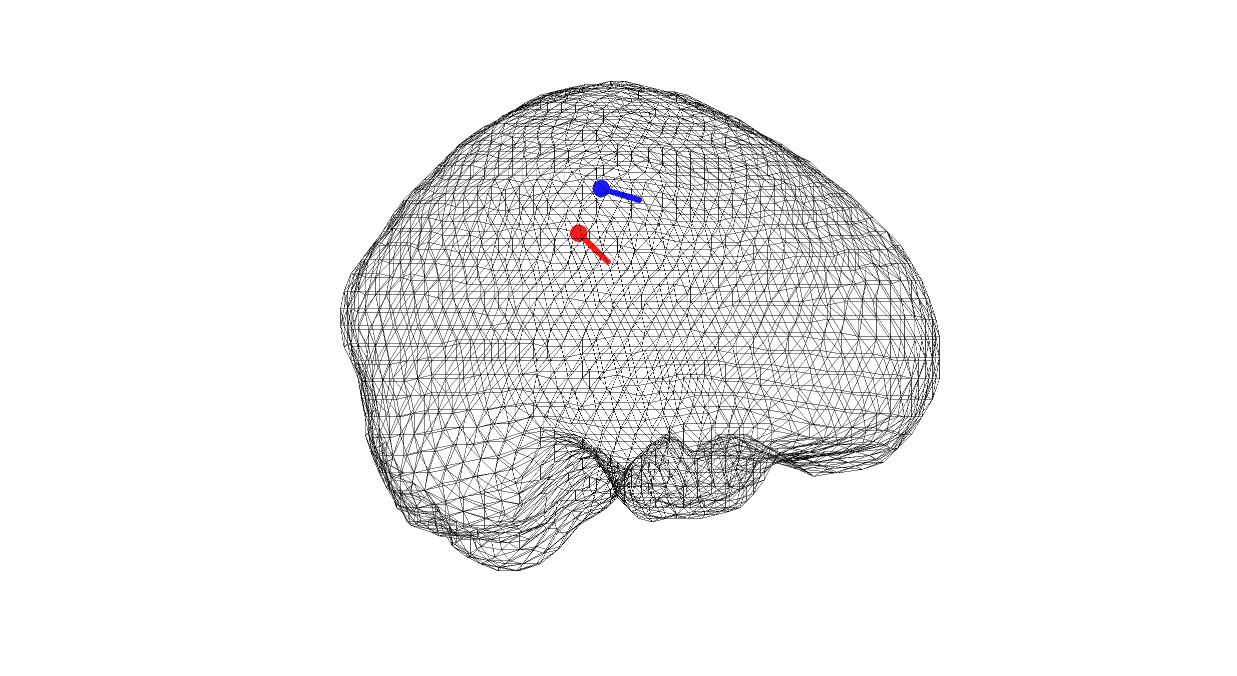
Figure 5. Comparison of a BEM and FEM dipole fit
Exercise 2
Can you think of reasons why the dipoles are at different locations?
Exercise 3
Changing parameters of the forward model influences the Inverse solutions. Play around with different parameters of the BEM forward model (e.g., changing conductivity values) and redo the inverse solution. If you need more input for this please ask us!
Summary and suggested further reading
In this tutorial we learned how solve the inverse problem. For this we used the preprocessed functional data and the forward model. The inverse techniques we used in this tutorial were “Dipole Fit” and “Minimum Norm Estimation”. We used both techniques with the different choices of for the forward model BEM and FEM.