Event-related potentials

Introduction

Event-related potentials can be used to reveal the activity that is time- and phase-locked to an event or stimulus. Furthermore, a contrast (or difference) between two ERPs can reveal the difference in the cortical processing between two different experimental conditions.

Prior to computing the ERP, we have to do some preprocessing: read the data into memory, segmenting the data around interesting events such as triggers, temporal filtering, artifact rejection and optionally rereferencing in the case of EEG. The ft_preprocessing function takes care of all these steps, i.e., it reads the data and applies the preprocessing options.

There are two alternative approaches for preprocessing, which especially differ in the amount of memory required. The first approach is to read all data from the file into memory, apply filters, and subsequently cut the data into interesting segments. The second approach is to first identify the interesting segments, only read those segments from the data file and apply the filters each segment. The remainder of this tutorial explains the second approach; it is in general more memory efficient also works for large data sets.

Note that the dataset in this tutorial is not particularly large; we could also have used the first approach. But we want to demonstrate how to work efficiently in general with large datasets with many trials where we are not interested in what happens in the breaks.

Both methods are compared in the preprocessing tutorial.

The dataset used in this tutorial

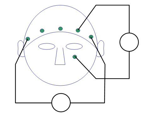
The eeg-language dataset was acquired by Irina Siminova in a study investigating semantic processing of stimuli presented as pictures, visually displayed text or as auditory presented words. Data was acquired with a 64-channel BrainProducts BrainAmp EEG amplifier from 60 scalp electrodes placed in an electrode cap, one electrode placed under the right eye; signals “EOGv” and “EOGh” are computed after acquisition using rereferencing. During acquisition all channels were referenced to the left mastoid and an electrode placed at the earlobe was used as the ground. Channels 1-60 correspond to electrodes that are located on the head, except for channel 53 which is located at the right mastoid. Channels 61, 62, 63 are not connected to an electrode at all. Channel 64 is connected to an electrode placed below the left eye. Hence we have 62 channels of interest: 60 for the scalp EEG electrodes plus one EOGH and one EOGV channel. More details on the experiment and data can be found here.

Procedure

In this tutorial the following steps will be taken:

Read the data using ft_definetrial and ft_preprocessing
Extract bipolar EOG channels with ft_preprocessing and get rid of reference channels with ft_selectdata. Combine EOG and data channels with ft_appenddata.
Visual artifact rejection with ft_databrowser and ft_rejectvisual.
Computing trial averages with ft_timelockanalysis.
Plotting ERPs with ft_topoplotER

Preprocessing

We are starting with a single-subject dataset that is available from our download server. During the workshop, you don’t have to download the data to your computer, it should already be present on the online MATLAB environment.

filename = 'language.vhdr'; % this also needs the corresponding .vmrk and .eeg file

Reading trials

Let us first look at the different trigger codes present in the dataset

cfg = [];
cfg.dataset             = filename;
cfg.trialdef.eventtype = '?';
dummy                   = ft_definetrial(cfg);

This will display the event types and values on screen. The trigger codes S112, S122, S132, S142 (animals) S152, S162, S172, S182 (tools) correspond to the presented visual stimuli. The trigger codes S113, S123, S133, S143 (animals) S153, S163, S173, S183 (tools) correspond to the presented auditory stimuli. These are the triggers we will select for now.

trigVIS = {'S112', 'S122', 'S132', 'S142', 'S152', 'S162', 'S172', 'S182'};
trigAUD = {'S113', 'S123', 'S133', 'S143', 'S153', 'S163', 'S173', 'S183'};

cfg = [];
cfg.dataset             = filename;
cfg.trialdef.eventtype  = 'Stimulus';
cfg.trialdef.eventvalue = [trigVIS trigAUD];
cfg.trialdef.prestim    = 0.5;
cfg.trialdef.poststim   = 0.8;
cfg                     = ft_definetrial(cfg);

After the call to ft_definetrial, the configuration structure cfg now not only stores the dataset name, but also contains a field cfg.trl with the definition of the segments of data that will be used for further processing and analysis. Each row in the trl matrix represents a single epoch-of-interest, and the trl matrix has at least 3 columns. The first column defines (in samples) the begin sample of each epoch with respect to how the data are stored in the raw datafile. The second column defines the end sample of each epoch, and the third column specifies the offset of the first sample within each epoch with respect to time 0 within that epoch.

disp(cfg)

disp(cfg.trl)

We will now read in the trials that were defined. For preprocessing this EEG data set, the choice of the reference has to be considered. During acquisition the reference channel of the EEG amplifier was attached to the left mastoid. We would like to analyze this data with a linked-mastoid reference (also known as an average-mastoid reference).

cfg.reref       = 'yes';
cfg.channel     = 'all';
cfg.implicitref = 'M1';         % the implicit (non-recorded) reference channel is added to the data
cfg.refchannel  = {'M1', '53'}; % the average of these will be the new reference, note that '53' corresponds to the right mastoid (M2)

Filtering options

cfg.lpfilter        = 'yes';
cfg.lpfreq          = 100;
cfg.demean          = 'yes';
cfg.baselinewindow  = [-inf 0];
data                = ft_preprocessing(cfg);

For consistency we will rename the channel with the name ‘53’ located at the right mastoid to ‘M2’.

chanindx = find(strcmp(data.label, '53'));
data.label{chanindx} = 'M2';

Extracting EOG channels

We now continue with rereferencing to extract the bipolar EOG signal from the data. For the vertical EOG we will use channel 50 and channel 64. For the horizontal EOG we will compute the difference between the potential recorded in channels 51 and 60.

Some EEG acquisition systems like the TMSi SAGA, the Biosemi systems, or the BrainProducts ActiChamp, allow for direct bipolar recording of ECG, EOG and EMG. The rereferencing step to obtain the EOG is therefore not required when working with those bipolar recordings.

Select the channels that we need for the vertical EOG

cfg              = [];
cfg.channel      = {'50' '64'};
cfg.reref        = 'yes';
cfg.implicitref  = []; % this is the default, we mention it here to be explicit
cfg.refchannel   = {'50'};
eogv             = ft_preprocessing(cfg, data);

only keep one channel, and rename it to EOGV

cfg              = [];
cfg.channel      = '64';
eogv             = ft_selectdata(cfg, eogv);
eogv.label       = {'eogv'};

Select the channels that we need for the horizontal EOG

cfg              = [];
cfg.channel      = {'51' '60'};
cfg.reref        = 'yes';
cfg.implicitref  = [];
cfg.refchannel   = {'51'};
eogh             = ft_preprocessing(cfg, data);

only keep one channel, and rename to it eogh

cfg              = [];
cfg.channel      = '60';
eogh             = ft_selectdata(cfg, eogh);
eogh.label       = {'eogh'};

We can now discard the channel corresponding to the electrode below the eye and add the bipolar-referenced EOGV and EOGH channels that we have just created.

Keep only the EEG channels

cfg         = [];
cfg.channel = {'all', '-61', '-62', '-63', '-64'}; % take all channels minus the ones specified
data        = ft_selectdata(cfg, data);

Append the EOGH and EOGV channel to the selected EEG channels

cfg  = [];
data = ft_appenddata(cfg, data, eogv, eogh);

Rather than rereferencing the EEG and the two EOG channels and renaming them subsequently, we could also have used the cfg.montage option in ft_preprocessing. The method of using a montage is explained here.

FieldTrip data structures are intended to be “lightweight”, in the sense that the internal MATLAB arrays can be transparently accessed. Have a look at the data as you read it into memory

>> data

data =

       hdr: [1x1 struct]
     label: {1x65 cell}
      time: {1x400 cell}
     trial: {1x400 cell}
   fsample: 500
sampleinfo: [400x2 double]
 trialinfo: [400x1 double]
       cfg: [1x1 struct]

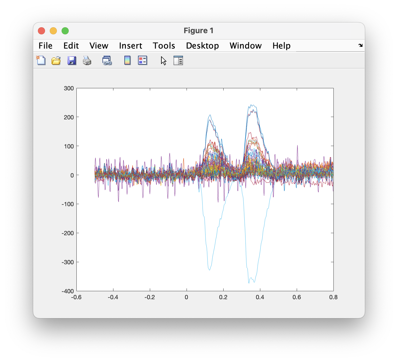
The fields in the raw data structure are explained in more detail in ft_dataype_raw. You can use the default MATLAB plot functions to show the EEG data for all channels in for example the first trial:

plot(data.time{1}, data.trial{1});

However, a more efficient way to quickly visualize and scroll through your data is to use ft_databrowser. That function also allows you to mark the time windows in which artifacts are present.

Visual artifacts detection

When using visual inspection to detect and reject artifacts, keep in mind that it is often a subjective decision to reject certain trials and to keep others. The type of artifacts to reject depends on the follow-up analysis you would like to do. For frequency analysis of power in the gamma band it is important to reject all trials with (high frequency) muscle artifacts, but for a ERP analysis it is more important to reject trials with (low frequency) drifts and eye artifacts.

It is important that you make your selection of trials blind to the experimental manipulation. e.g., in an oddball experiment when you have many standards and few oddballs, you might be tempted to be more strict on the standards and more lenient on the oddballs. This would result in more remaining artifacts in your oddball condition, which could cause a trivial difference in the ERP waveforms.

So you should apply the same criteria for artifact rejection to all your experimental conditions.

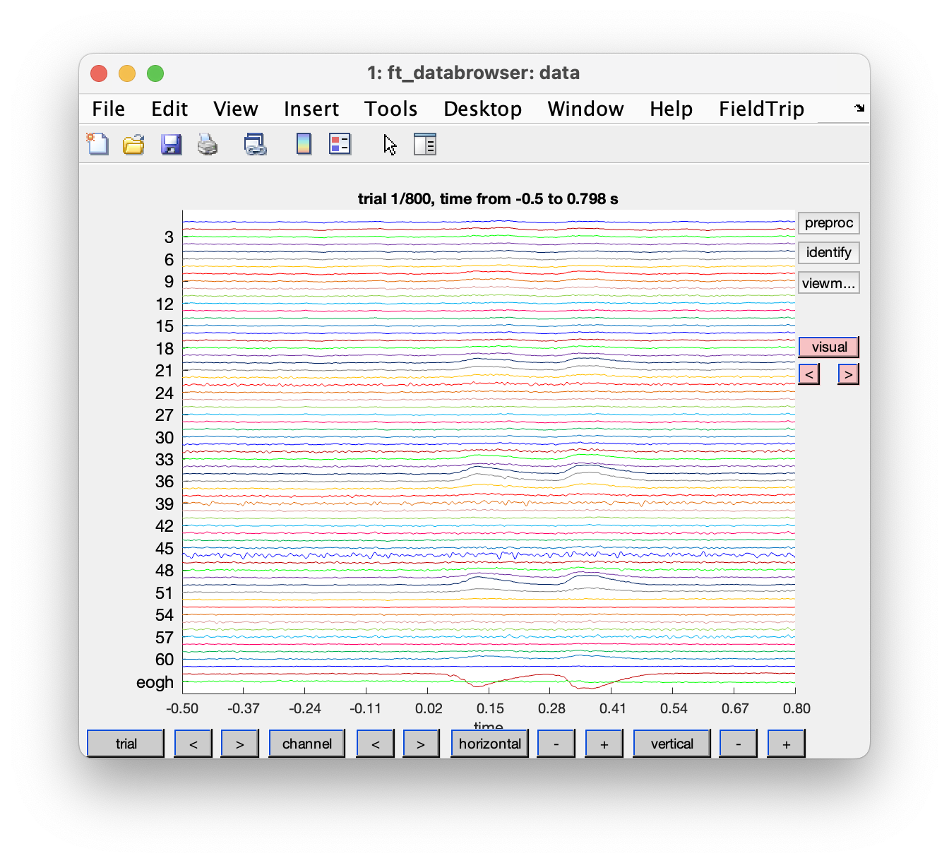
To get a first impression of our data quality we will use ft_databrowser to look at our individual trials. This is a good option if you want to quickly browse your data, as it takes both continuous and segmented data as inputs. With ft_databrowser you can display all channels at the same time to inspect non-systematic artifacts such as blinks or electrode movement.

cfg          = [];
cfg.viewmode = 'vertical';
artfct       = ft_databrowser(cfg, data)

Exercise 1

Skip through a couple of data segments and see if you can already spot some artifacts. Use the buttons to mark an artifact. Are there any bad channels in this dataset?

As you might have noticed it is easy to mark segments with ft_databrowser, but it is not possible to mark channels as bad; also looking at each trial individually and then clicking with the mouse to go to the next is not always very efficient.

Display one trial at a time

Another option for visual artifact detection is ft_rejectvisual. This function allows you to inspect data that has been segmented into trials and identify either bad trials or bad channels. It allows you to browse through large amounts of data in a single figure by either showing all channels at once (per trial), or showing all trials at once (per channel), or by showing a summary of all channels and trials.

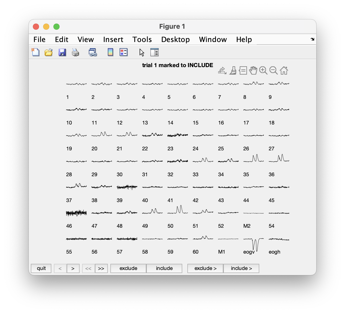
We will first call ft_rejectvisual with all channels at once. This corresponds more or less to the way that ft_databrowser displays the data (one trial at the time), but now we can see individual channels better and can mark channels that are bad.

cfg          = [];
cfg.method   = 'trial';
data_clean   = ft_rejectvisual(cfg, data);

To mark a channel that is bad, you have to click in the figure on that specific channel. Clicking the channel once more toggles it back to good. To mark the whole trial as bad, you have to click on the “bad” button at the bottom of the figure. Click through the trials using the > button to inspect each trial.

Please click on channel 46 to exclude that from further analysis. It appears to be noisy in all trials.

Exercise 2

Can you spot which channels are noisier than others? Using the mouse and clicking, you can select channels that you want to remove from the data.

The ft_rejectvisual function directly returns the clean data with the bad channels and trials removed and you do not have to call ft_rejectartifact or ft_rejectcomponent. We could continue working with the cleaned data, but for now we will only save the list of channel names of the the bad channels and continue with our data inspection.

bad_chan = setdiff(data.label, data_clean.label);

Display one channel at a time

Next we will use ft_rejectvisual to display all trials for a single channel; this is helpful to identify whether the channel is noisy in general, or becomes bad at a certain time during the experiment, or only has some glitches. It is also helpful to inspect the EOG channels to identify trials that have eye blinks or eye movements. Since we removed some bad trials, the cleaned data would already have fewer trials than the original.

cfg          = [];
cfg.method   = 'channel';
cfg.channel  = {bad_chan{:},'eogv','eogh'};
data_clean   = ft_rejectvisual(cfg, data);

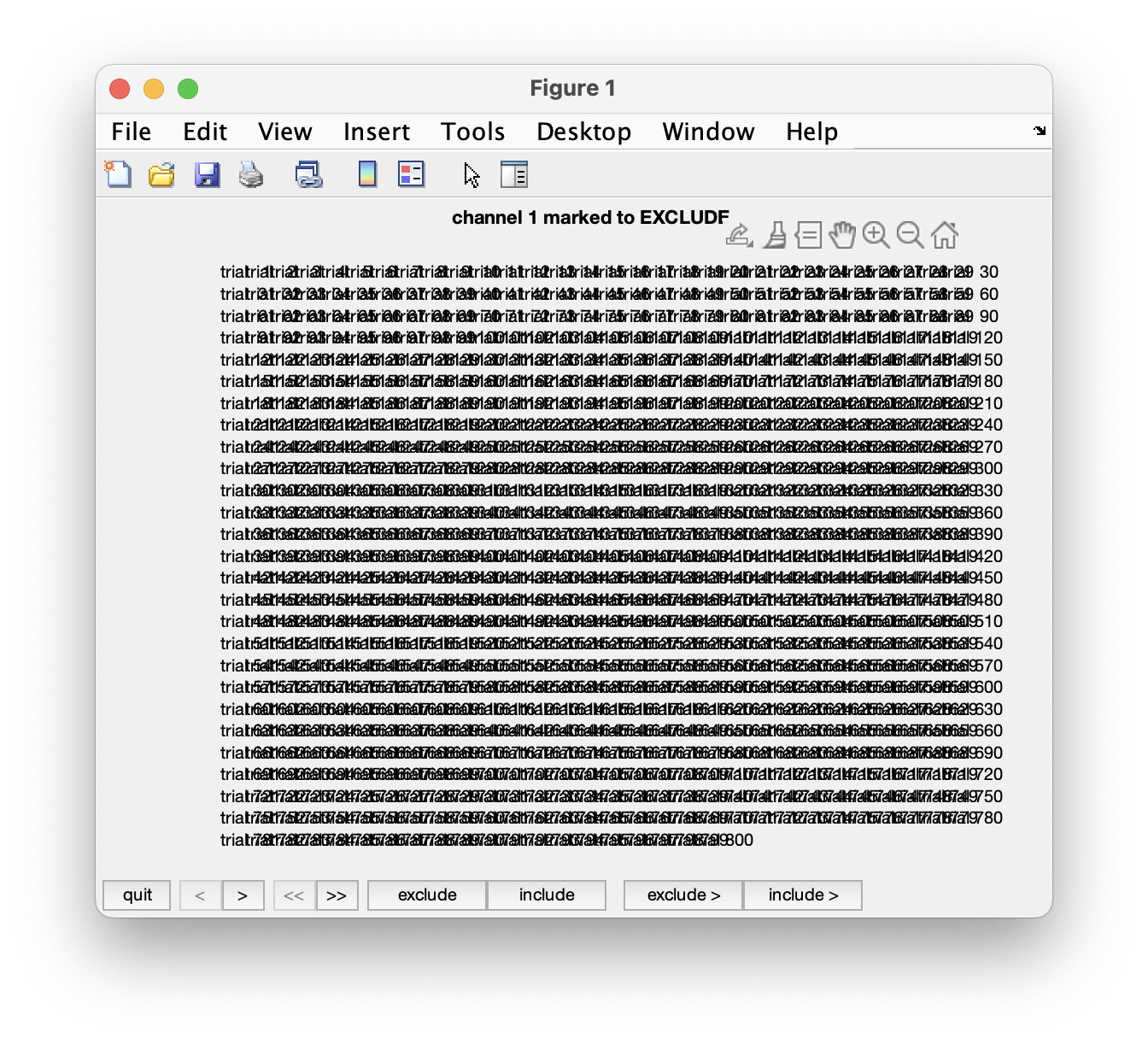
Note that this will be not so effective if you have a small screen and many trials. This dataset has 800 trials, which means that 800 small plots are made, each with a timecourse. On a small screen you will not be able to make out the timecourses, so you cannot judge whether there are artifacts or not. Also there are many trials to judge, which can take a long time.

If we have a large enough screen and can see the timecourses in the trial, we can identify and store the trial numbers that have blinks. We are using the trialinfo field for this, which contains the begin and end sample relative to the original data file.

bad_trial = ismember(data.sampleinfo(:,1), setdiff(data. sampleinfo(:,1), data_clean.sampleinfo(:,1)));

Display a summary

Finally we will call ft_rejectvisual one more time in ‘summary’ mode. This option is the fastest to identify either trials or channels that are noisy.

cfg          = [];
cfg.method   = 'summary';
cfg.channel  = 'all';
cfg.trials   = ~bad_trial; % exclude the trials that we already identified as bad
data_clean   = ft_rejectvisual(cfg, data);

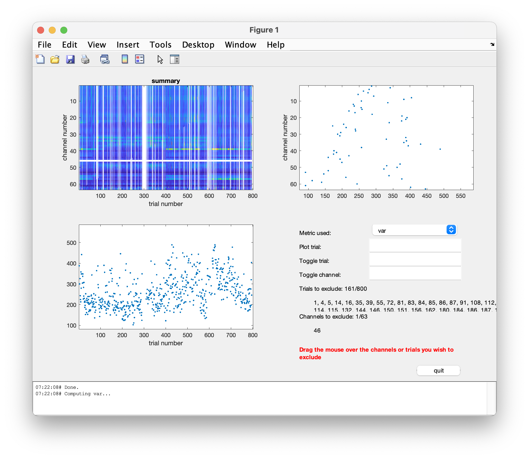
Exercise 3

Which channels show the most variance? Why is that?

If you would like to keep track of which trials you reject, keep in mind that the trial numbers change when you call ft_rejectvisual more than once, or if you use the cfg.trials option for selection. If you want to keep track which data you rejected, it is best look at the sample numbers in the trialinfo field. These sample numbers always refer to the original EEG data file.

Inspect cleaned data

Now that we have identified artifacts using different visual inspection approaches, we will use ft_databrowser again to inspect the data with bad trials marked as such. For this we first compare the sampleinfo between the original and the clean data structure.

bad_samples = data.sampleinfo(ismember(data.sampleinfo(:,1), setdiff(data.sampleinfo(:,1), data_clean.sampleinfo(:,1))),:);

cfg = [];
cfg.viewmode                  = 'vertical';
cfg.artfctdef.visual.artifact = bad_samples;
cfg_artif = ft_databrowser(cfg, data);

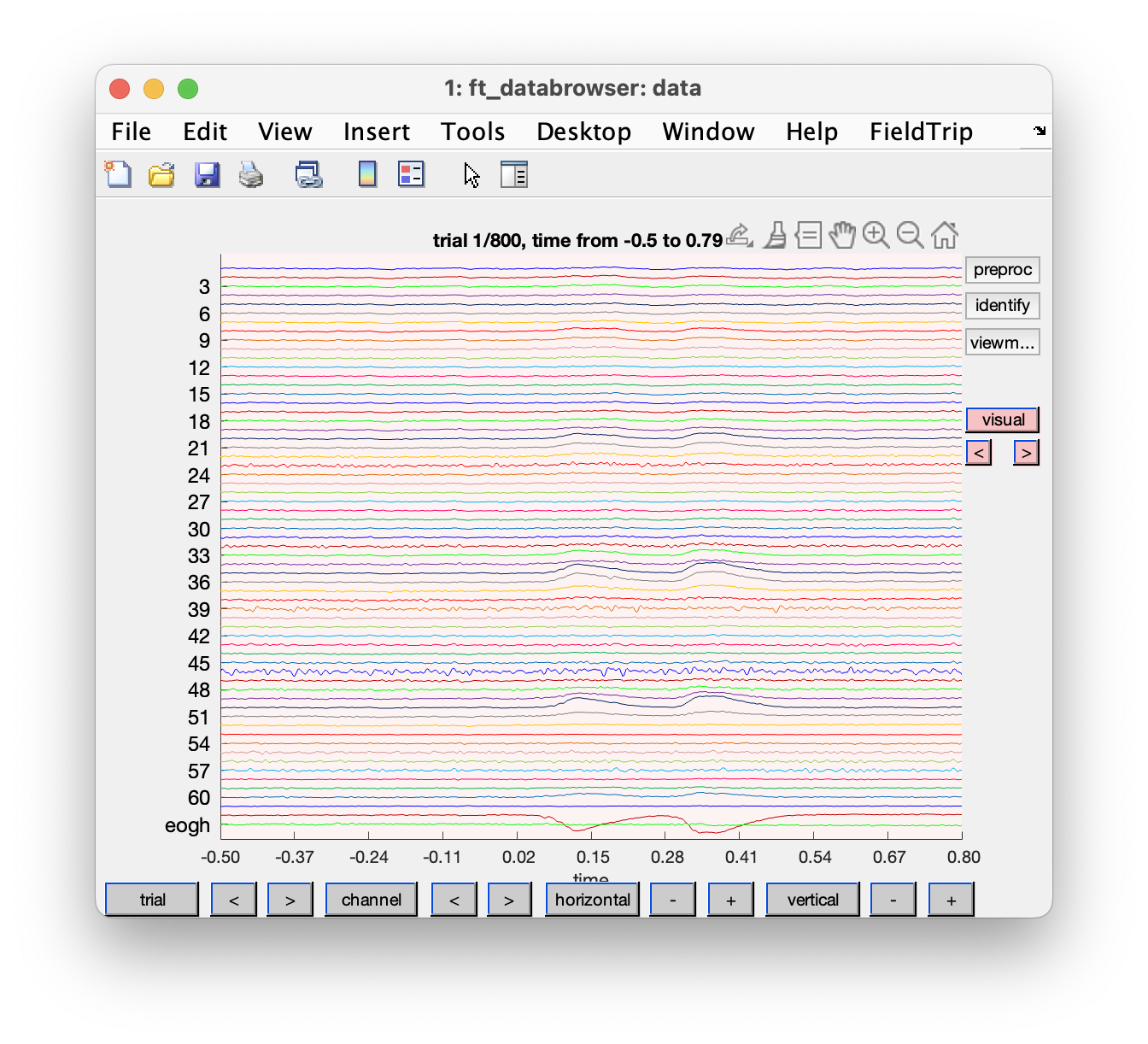
If the cleaning with ft_rejectvisual was not sufficient yet, you can continue to mark trials or data segments as artifacts within ft_databrowser. The updated artifact definition will be saved in the cfg_artif output and you can subsequently reject those artifacts using ft_rejectartifact.

Computing and plotting the ERPs

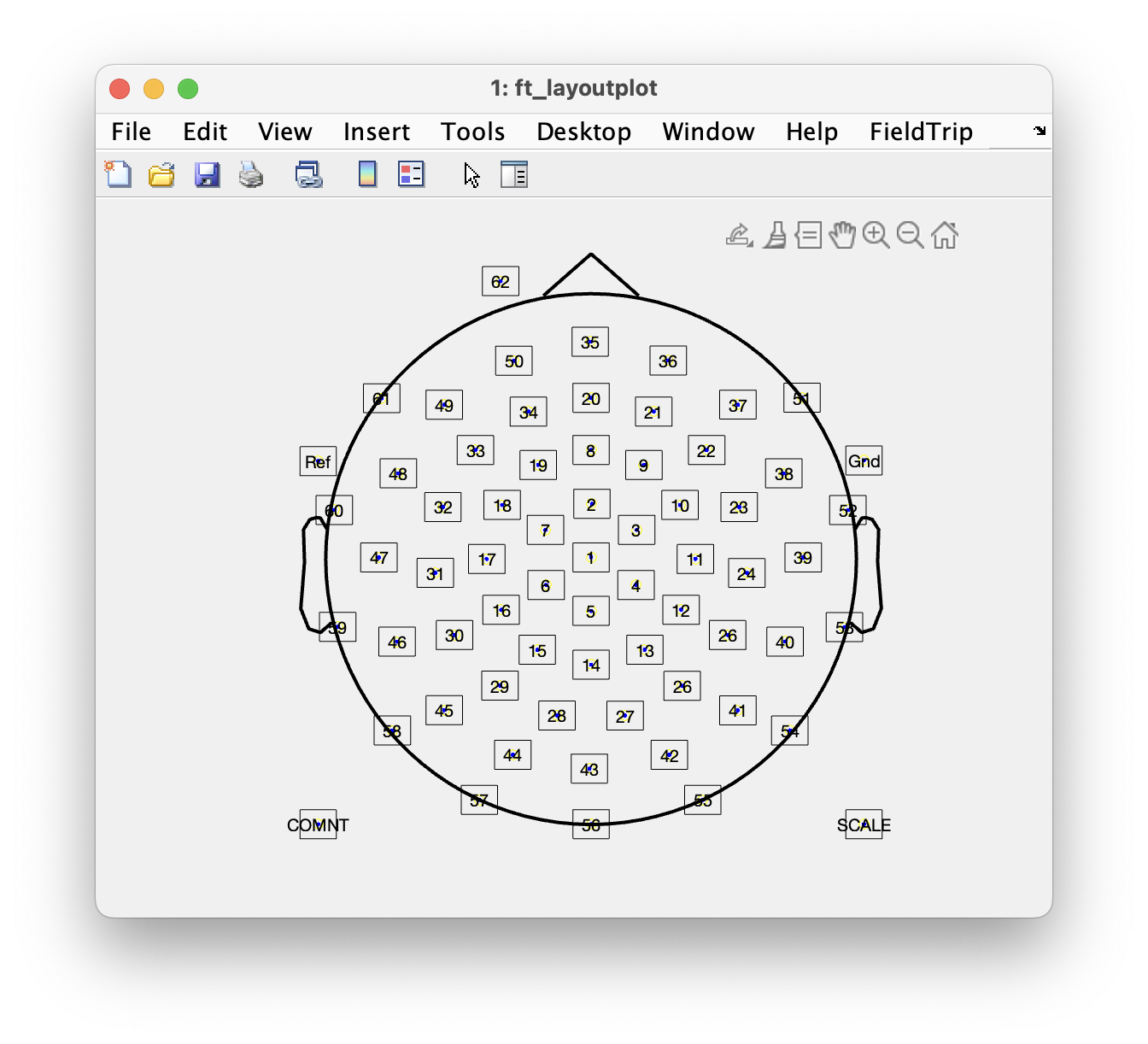
Channel layout

For topographic plotting and for some other follow-up analyses it is necessary to know precisely where the electrodes were positioned on the scalp. The topographical arrangement of the electrodes in an EEG cap is not the same in all caps, and even for a standard placement system like 10-20 or 10-20 might vary a bit between manufacturers. You can use the acquisition system with different caps, and the number and position of electrodes can be adjusted depending on the experimental question. In the current data, a cap with a so-called equidistant electrode layout was used for a 64-channel active electrode system (BrainVision ActiCap).

The electrode positions are in general not recorded during EEG measurements (although, see this tutorial) and are hence not stored in the EEG dataset. For plotting you have to use a layout file; this is a .lay or a .mat file that contains the 2-D positions of the channels on screen. FieldTrip provides a number of template layouts for different EEG caps in the fieldtrip/template/layout directory. See the template layouts to get an overview of some electrode cap layouts. It is also possible to create custom layouts for your own EEG cap, see ft_prepare_layout and the layout tutorial.

cfg = [];
cfg.layout = 'easycapM10.mat';
ft_layoutplot(cfg)

Trial-average

We will now compute the ERPs for two conditions corresponding to visual and auditory stimulus presentation.

For each trial, the condition information is kept with the data structure in data.trialinfo. We use ft_timelockanalysis to compute the ERPs and average only those trials in which the trigger code corresponds to the condition of interest (i.e. visual or auditory).

cfg = [];
cfg.trials = ismember(data_clean.trialinfo, [112, 122, 132, 142]);
timelockVIS = ft_timelockanalysis(cfg, data_clean);

cfg = [];
cfg.trials = ismember(data_clean.trialinfo, [113, 123, 133, 143]);
timelockAUD = ft_timelockanalysis(cfg, data_clean);

Exercise 4

Inspect the resulting data structure after ft_timelockanalysis.

Which fields have been added and what information do they contain? The fields in the data structure are explained in more detail in ft_datatype_timelock.

We will now use ft_topoplotER to plot both conditions. You can interact with the figure by selecting certain channels or time windows using your mouse, and going back and forth between the topographic and time representation of the data.

cfg = [];
cfg.layout      = 'easycapM10.mat';
cfg.interactive = 'yes';
cfg.baseline    = [-0.2 0];
ft_topoplotER(cfg, timelockAUD, timelockVIS)

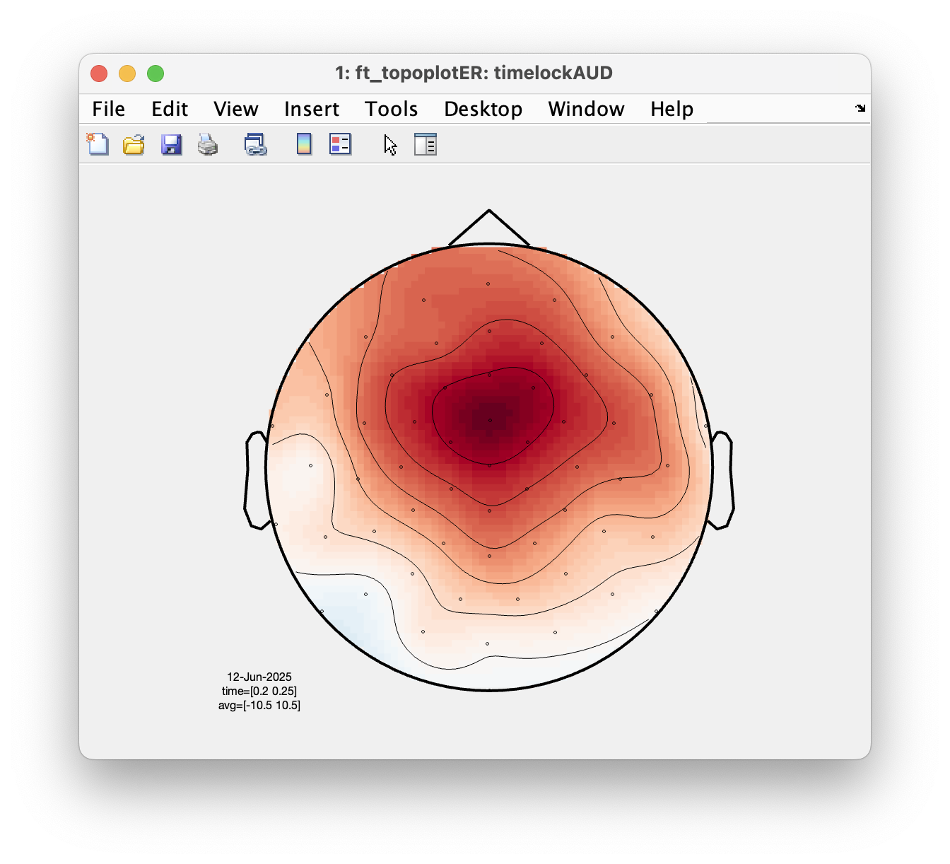
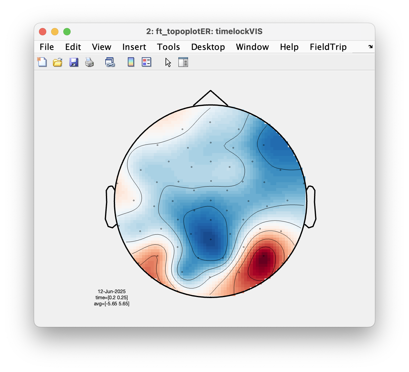
Exercise 5

Select the time window where the conditions differ the most. Do the topographies look as you would expect?

Next steps

Following the computation of ERPs, FieldTrip offers many more functions to continue analyzing your data. You can use ft_math to compute difference waves, ft_timelockstatistics to run statistics on your ERP effect, compute group level averages with ft_timelockgrandaverage or explore different ways of visualizing, i.e. ft_multiplotER etc.

Exercise 6

The following code allows you to compute at the ERP difference waves.

cfg = [];
cfg.operation = 'x1-x2';
cfg.parameter = 'avg';
difference = ft_math(cfg, timelockAUD, timelockVIS);

This in principle does the same as

difference     = timelockAUD;                        % copy one of the structures
difference.avg = timelockAUD.avg - timelockVIS.avg;  % compute the difference ERP

but ft_math will keep provenance (i.e. historical information) in the output cfg structure, whereas if you do it by hand you will loose the information, which might make it more difficult later in your analysis to figure out what you exactly did to your data.