workshop / ohbm2018 / preprocessing /
Preprocessing of EEG and MEG data
Introduction
This tutorial describes how to define epochs-of-interest (trials) from your recorded EEG-data, and how to apply the different preprocessing steps. This tutorial also shows you how to average your data for a specific experiment (electric wrist stimulation on the right hand).
This tutorial does the preprocessing and segmenting in a single step. If you are interested in how to do preprocessing on your continuous data prior to segmenting it into trials, you can check the Preprocessing - Reading continuous data tutorial.
This tutorial contains the hands-on material of the BACI workshop and is complemented by this lecture.
Background
Preprocessing of MEG or EEG data refers to reading the data into memory, segmenting the data around interesting events such as triggers, temporal filtering and (optionally) rereferencing. The ft_preprocessing function takes care of all these steps, i.e., it reads the data and applies the preprocessing options.
There are largely two alternative approaches for preprocessing, which especially differ in the amount of memory required. The first approach is to read all data from the file into memory, apply filters, and subsequently cut the data into interesting segments. The second approach is to first identify the interesting segments, read those segments from the data file and apply the filters to those segments only. The remainder of this tutorial explains the second approach, as that is the most appropriate for large data sets such as the MEG data used in this tutorial. The approach for reading and filtering continuous data and segmenting afterwards is explained in another tutorial.
Preprocessing involves several steps including identifying individual trials from the dataset, filtering and artifact rejections. This tutorial covers how to identify trials using the trigger signal. Defining data segments of interest can be done
- according to a specific trigger channel
- according to your own criteria when you write your own trial function, e.g., for conditional trigger sequences, or by detecting the onset of movement in an EMG channel
Both depend on ft_definetrial. The output of ft_definetrial is a configuration structure containing the field cfg.trl. This is a matrix representing the relevant parts of the raw datafile which are to be selected for further processing. Each row in the trl matrix represents a single epoch-of-interest, and the trl matrix has 3 or more columns. The first column defines (in samples) the beginpoint of each epoch with respect to how the data are stored in the raw datafile. The second column defines (in samples) the endpoint of each epoch, and the third column specifies the offset (in samples) of the first sample within each epoch with respect to timepoint 0 within that epoch. The subsequent columns can be used to keep information about each trial.
If you do not specify your own trial function, the 4th column will by default contain the trigger value. When you use your own trial function, you can add any number of extra columns to the trl matrix. These will be added to the data in the .trialinfo field. This is very handy if you want to add information of e.g., response-buttons, response-times, etc., to each trial. As you will see, we will use this functionality to preprocess both the standard and deviant tones together, and then separating them later for averaging.
Description of the experimental data
For the source reconstruction workshop we recorded a single subject to allow you to work through all basic steps involved in EEG/MEG analysis: from event-related averaging to forward and inverse problem.
Somatosensory Evoked Potentials/Fields (SEPs/SEFs)
Primary somatosensory cortex (SI) is part of the postcentral gyrus of the human brain. SI consists of Brodmann areas 1, 2, and 3.
Here, the response of interest is the well-known P20/N20 complex (or component) which is generated in area 3b (part of the Brodmann areas 3). The generators of this area are mainly focal not too deep and mainly tangentially oriented (Allison et al. 1989).
Estimation of the P20/N20 component
The median nerve of the subject’s right wrist was stimulated using square electrical pulses with 0.5 ms duration. The stimulus strength was adjusted to see a clear movement of the thumb. The inter-stimulus interval was varied randomly between 350 to 450 ms to avoid habituation and to obtain a clear pre-stimulus interval. A reduction in stimulus artifacts was achieved by reversing the polarity of the stimulation during the second half of the measurement.
Triggers
The EEG system records event-triggers in separate channels. These channels are recorded simultaneously with the data channels, and at the same sampling rate. The onset can therefore be precisely timed with respect to the data. The following trigger codes can be used for the analysis we will be doing during the worksho
- Onset of standard stimulus: 2
- Name of standard stimulus : rightArm
Data
- Data was sampled at 1200Hz.
- 74 channel EEG. The reference was placed on the FCz channel.
- Electrocardiogram (ECG) was recorded as a bipolar recording from the collarbones.
- Horizontal EOG(1) electrodes were placed just next to the left and right eye. Vertical EOG(2) were placed above and below the left eye.
- 10 minutes of recording (5 minutes with normal polarity of the electric pulses and 5 with inverse polarity of the electric pulses)
Preprocessing and averaging EEG & MEG
Procedure
The following steps are taken in the EEG section of the tutorial:
- Define segments of data of interest (the trial definition) using ft_definetrial
- Read the data into Matlab using ft_preprocessing
- Clean the data in a semi-automatic way using ft_rejectvisual
- Compute event-related fields using ft_timelockanalysis
- Compute global mean field power using ft_globalmeanfield
- Visualize the results using ft_topoplotER, and ft_multiplotER
Reading and preprocessing the interesting trials
We start with the trial definition using ft_definetrial and ft_preprocessing.
data_name              = 'subject01.ds';        % define the data path and its name

% Read events
cfg                    = [];
cfg.trialdef.prestim   = 0.1;                   % in seconds
cfg.trialdef.poststim  = 0.2;                   % in seconds
cfg.trialdef.eventtype = 'rightArm';            % get a list of the available types
cfg.dataset            = data_name;             % set the name of the dataset
cfg_tr_def             = ft_definetrial(cfg);   % read the list of the specific stimulus

% segment data according to the trial definition
cfg                    = [];
cfg.dataset            = data_name;
cfg.channel            = 'eeg1010';             % define channel type
data_eeg               = ft_preprocessing(cfg); % read raw data
data_eeg               = ft_redefinetrial(cfg_tr_def, data_eeg);

cfg                    = [];
cfg.dataset            = data_name;
cfg.channel            = 'MEG';             % define channel type
data_meg               = ft_preprocessing(cfg); % read raw data
data_meg               = ft_redefinetrial(cfg_tr_def, data_meg);
We will filter the data using ft_preprocessing around the frequency spectrum of interest and eliminate the power line noise before calculating the SEP/SEFs with ft_timelockanalysis.
cfg                = [];
cfg.hpfilter       = 'yes';           % enable high-pass filtering
cfg.lpfilter       = 'yes';           % enable low-pass filtering
cfg.hpfreq         = 20;              % set up the frequency for high-pass filter
cfg.lpfreq         = 250;             % set up the frequency for low-pass filter
cfg.dftfilter      = 'yes';           % enable notch filtering to eliminate power line noise
cfg.dftfreq        = [50 100 150];    % set up the frequencies for notch filtering
cfg.baselinewindow = [-0.1 -0.02];    % define the baseline window
data_eeg           = ft_preprocessing(cfg, data_eeg);
data_meg           = ft_preprocessing(cfg, data_meg);
The output of data is the structure data which has the following fields:
data_eeg =
         hdr: [1x1 struct]
        elec: [1x1 struct]
     fsample: 1200
  sampleinfo: [1198x2 double]
       trial: {1x1198 cell}
        time: {1x1198 cell}
       label: {74x1 cell}
         cfg: [1x1 struct]

data_meg =
         hdr: [1x1 struct]
       trial: {1x1198 cell}
        time: {1x1198 cell}
        elec: [1x1 struct]
     fsample: 1200
        grad: [1x1 struct]
       label: {271x1 cell}
  sampleinfo: [1198x2 double]
         cfg: [1x1 struct]
In the data structure of data_meg/data_eeg we see it still contains elec/grad. With the following code we remove elec/grad from the structure, otherwise we encounter problems in the later step of processing.
data_meg = rmfield(data_meg, 'elec')
data_eeg = rmfield(data_eeg, 'grad')
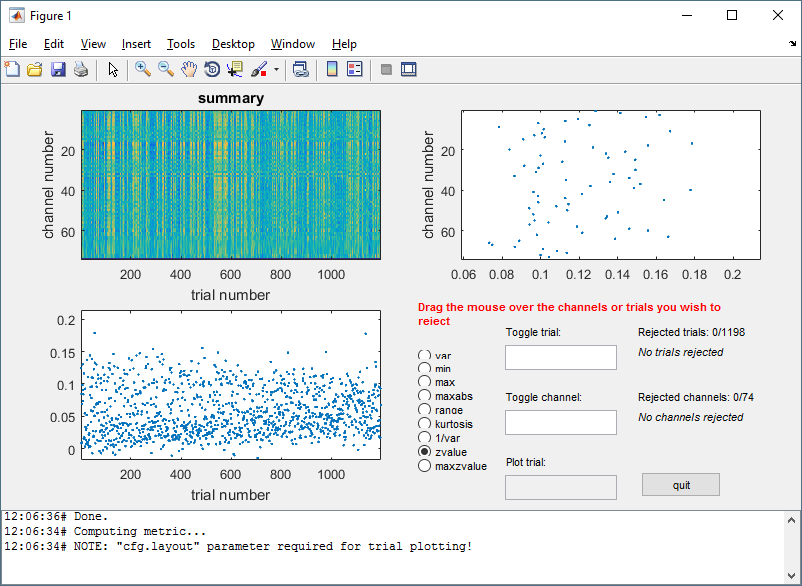
We will use ft_rejectartifact to clean the data of bad trials (and perhaps channels). We use only the ‘zvalue’ criterion to eliminate bad trials (or channels). You can play around with other criterion where you can reject trial.
cfg        = [];
cfg.metric = 'zvalue';  % use by default zvalue method
cfg.method = 'summary'; % use by default summary method

data_eeg       = ft_rejectvisual(cfg,data_eeg);
data_meg       = ft_rejectvisual(cfg,data_meg);
Figure 1: Example of visual rejection.
Somatosensory Evoked Potentials/Fields (SEPs/SEFs)
Timelockanalysis
The function ft_timelockanalysis averages all the trials into a single trial. It requires preprocessed data, i.e. what we just did.
The trials belonging to one condition will now be averaged with the onset of the stimulus time aligned to the zero-time point. This is done with the function ft_timelockanalysis. The input to this procedure is the data structure generated by ft_preprocessing.
cfg                   = [];
cfg.preproc.demean    = 'yes';    % enable demean to remove mean value from each single trial
cfg.covariance        = 'yes';    % calculate covariance matrix of the data
cfg.covariancewindow  = [-0.1 0]; % calculate the covariance matrix for a specific time window
EEG_avg               = ft_timelockanalysis(cfg, data_eeg);
MEG_avg               = ft_timelockanalysis(cfg, data_meg);
Data rereferencing
We should rereference the averaged EEG data for later use in the inverse problem, inverse problem.
cfg               = [];
cfg.reref         = 'yes';
cfg.refchannel    = 'all';
cfg.refmethod     = 'avg';
EEG_avg           = ft_preprocessing(cfg,EEG_avg);
Don’t forget to save the time locked data.
save MEG_avg MEG_avg
save EEG_avg EEG_avg
Global Mean Field Power
Global Mean Field Power (GMFP) is a measure first introduced by Lehmann and Skandries (1979), used by, for example, Esser et al. (2006) as a measure to characterize global EEG activity.
GMFP can be calculated using the following formula (from Esser et al. (2006))
where t is time, V is the voltage at channel i and K is the number of channels.
FieldTrip has a built-in function to calculate the GMFP; ft_globalmeanfield. This function requires timelocked data as input. We will use similar preprocessing as applied in Esser et al. (2006).
% global mean field power calculation for visualization purposes
cfg = [];
cfg.method = 'amplitude';
EEG_gmfp = ft_globalmeanfield(cfg, EEG_avg);
MEG_gmfp = ft_globalmeanfield(cfg, MEG_avg);
Plotting the results of EEG and MEG
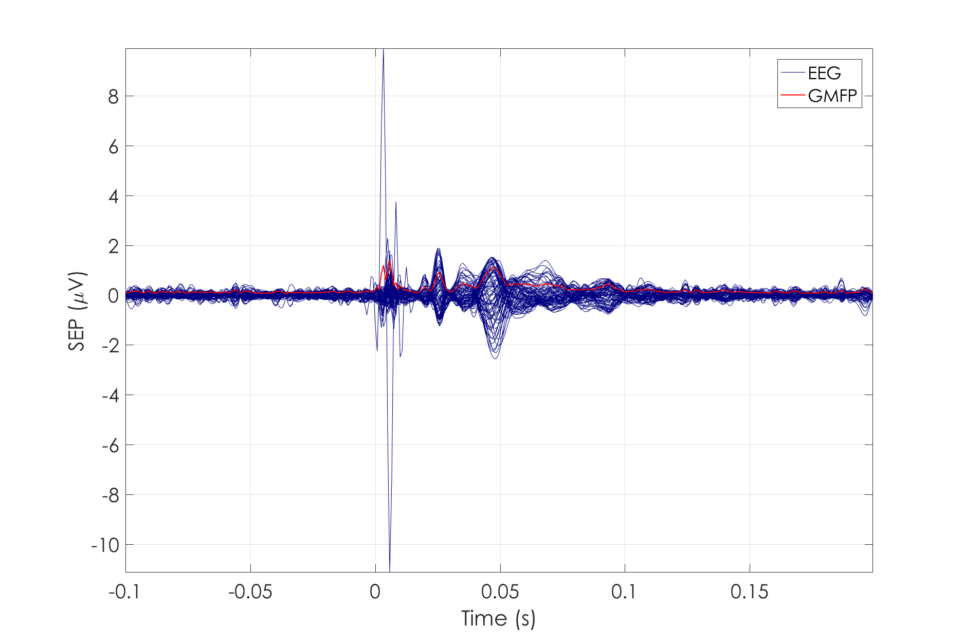
Using the plot functions ft_topoplotER and ft_multiplotER you can plot the average of the trials. You can find information about plotting also in the Plotting data at the channel and source level tutorial. Furthermore, we use the below script to visualize single trial with global mean field power and we find the time of interest and we save it together with the EEG_avg.
figure

pol = -1;     % correct polarity
scale = 10^6; % scale for eeg data micro volts

signal_EEG = scale * pol * EEG_avg.avg; % add single trials in a new value

% plot single trial together with global mean field power
h1 = plot(EEG_avg.time,signal_EEG,'color',[0,0,0.5]);
hold on;
h2 = plot(EEG_avg.time,scale*EEG_gmfp.avg,'color',[1,0,0],'linewidth',1);
Figure 2: Representation of single trial (blue) and the global mean field power of EEG (red).
figure

pol = -1;     % correct polarity
scale = 10^6; % scale for eeg data micro volts

signal_MEG = scale * pol * MEG_avg.avg; % add single trials in a new value

% plot single trial together with global mean field power
h1 = plot(MEG_avg.time,signal_MEG,'color',[0,0,0.5]);
hold on;
h2 = plot(MEG_avg.time,scale*MEG_gmfp.avg,'color',[1,0,0],'linewidth',1);
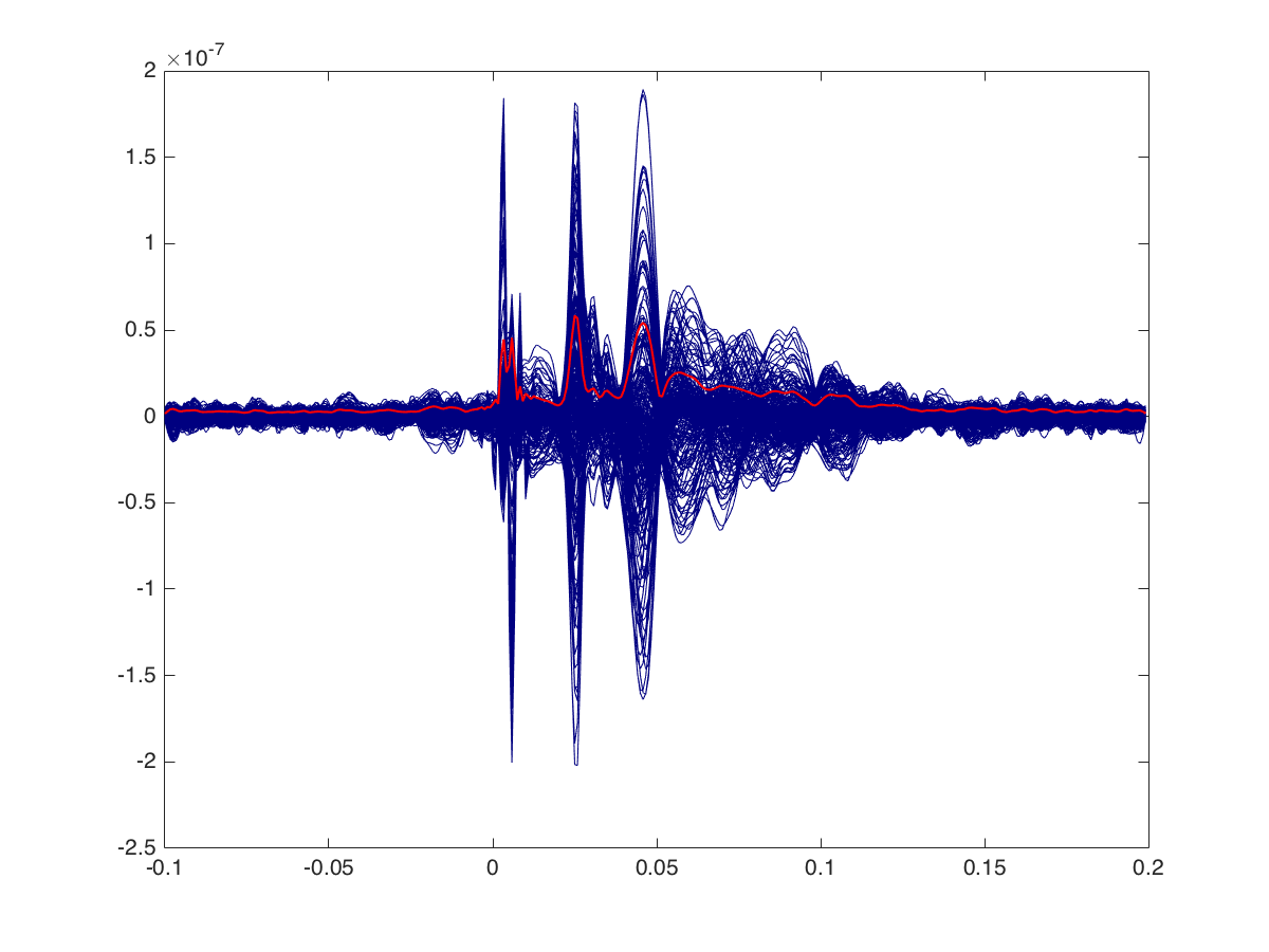
Figure 3: Representation of single trial (blue) and the global mean field power of MEG (red).
We set up values to create the image you observe before for EEG.
mx = max(max(signal_EEG));
mn = min(min(signal_EEG));

% select time of interest for the source reconstruction later on
idx = find(EEG_avg.time>0.024 & EEG_avg.time<=0.026);
toi = EEG_avg.time(idx);

[mxx,idxm] = max(max(abs(EEG_avg.avg(:,idx))));
EEG_toi_mean_trial = toi(idxm);
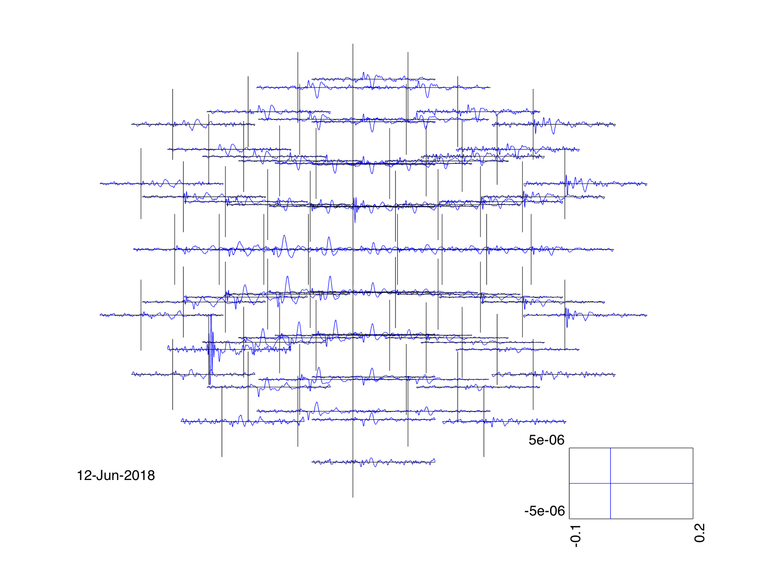
Use ft_multiplotER to plot all sensors in one figure:
cfg          = [];
cfg.fontsize = 6;
cfg.layout   = 'elec1010.lay';
cfg.fontsize = 14;
cfg.ylim     = [-5e-6 5e-6];
cfg.xlim     = [-0.1 0.2];

figure
ft_multiplotER(cfg, EEG_avg);

set(gcf, 'Position',[1 1 1200 800])
print -dpng baci_sep_multiplotER.png
Figure 4: Use of ft_multiplotER for representation of the single trial according to the EEG cap.
And now we create it for MEG
mx = max(max(signal_MEG));
mn = min(min(signal_MEG));

% select time of interest for the source reconstruction later on
idx = find(EEG_avg.time>0.024 & EEG_avg.time<=0.026);
toi = EEG_avg.time(idx);

[mxx,idxm] = max(max(abs(EEG_avg.avg(:,idx))));
MEG_toi_mean_trial = toi(idxm);
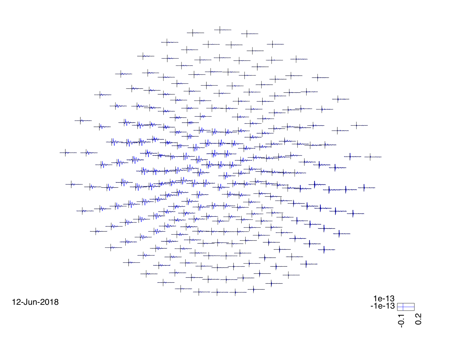
Use ft_multiplotER to plot all sensors in one figure:
cfg          = [];
cfg.fontsize = 6;
cfg.layout   = 'CTF275.lay';
cfg.fontsize = 14;
cfg.ylim     = [-1e-13 1e-13];
cfg.xlim     = [-0.1 0.2];

figure
ft_multiplotER(cfg, MEG_avg);

set(gcf, 'Position',[1 1 1200 800])
print -dpng baci_sef_multiplotER.png
Figure 5: Use of ft_multiplotER for representation of the single trial according to the EEG cap.
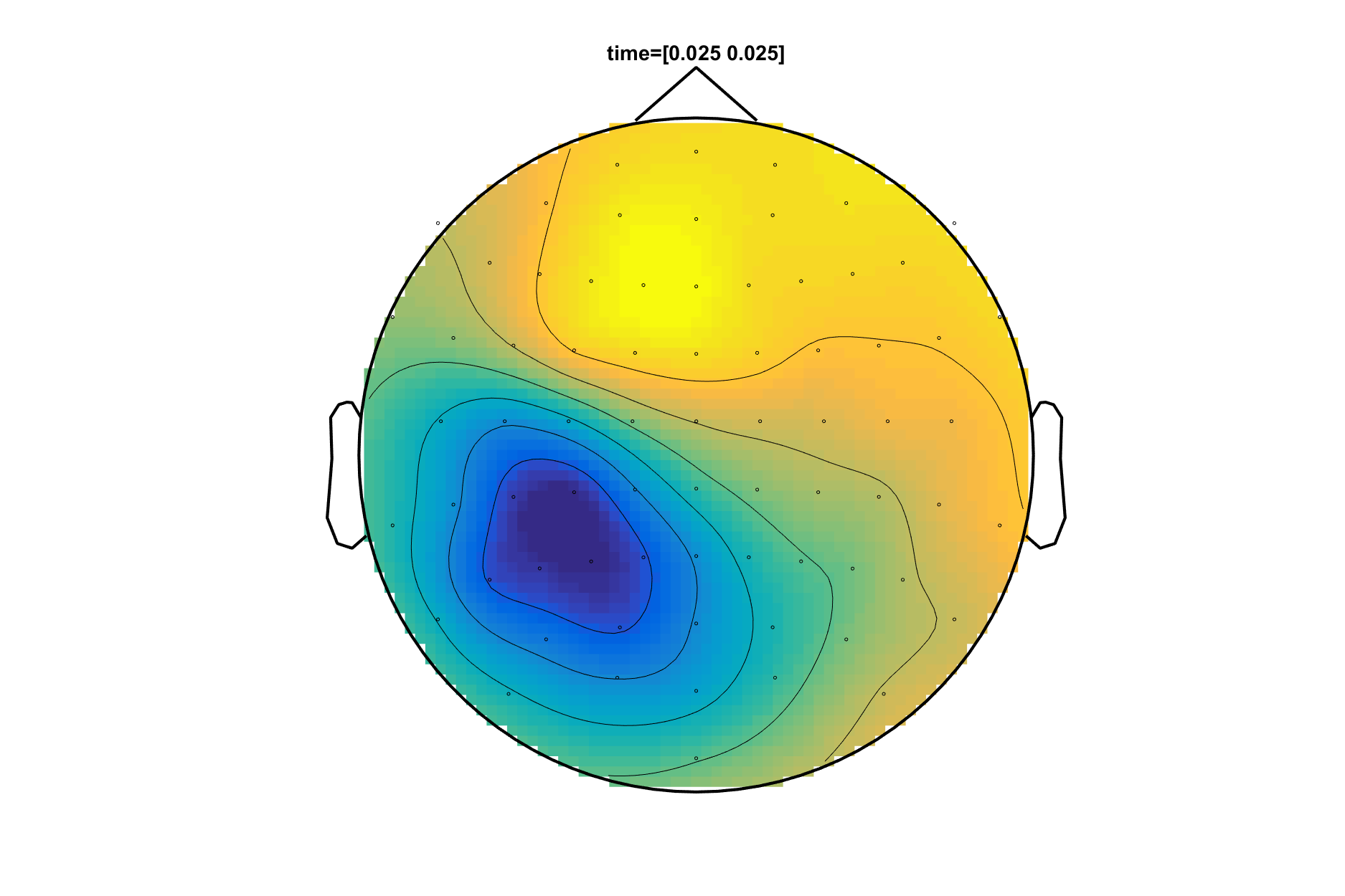
Use ft_topoplotER to plot the topographic distribution over the head:
cfg            = [];
cfg.zlim       = 'maxmin';
cfg.comment    = 'xlim';
cfg.commentpos = 'title';
cfg.xlim       = [EEG_toi_mean_trial EEG_toi_mean_trial+0.01*EEG_toi_mean_trial];
cfg.layout     = 'elec1010.lay';
cfg.fontsize   = 14;

figure
ft_topoplotER(cfg, EEG_avg);

set(gcf, 'Position',[1 1 1200 800])
print -dpng baci_sep_topo.png
Figure 6: Representation of the P20/N20 component using the function, ft_topoplotER.
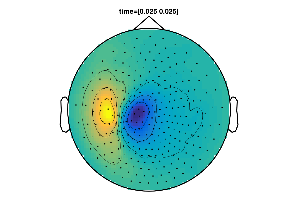
Use ft_topoplotER to plot the topographic distribution over the head:
cfg            = [];
cfg.zlim       = 'maxmin';
cfg.comment    = 'xlim';
cfg.commentpos = 'title';
cfg.xlim       = [MEG_toi_mean_trial MEG_toi_mean_trial+0.01*MEG_toi_mean_trial];
cfg.layout     = 'CTF275.lay';
cfg.fontsize   = 14;

figure
ft_topoplotER(cfg, MEG_avg);

set(gcf, 'Position',[1 1 1200 800])
print -dpng baci_sef_topo.png
Figure 7: Representation of the P20/N20 component using the function, ft_topoplotER.
Summary and suggested further reading
In this tutorial we learned how to look at EEG data, define trials based on trigger codes, preprocess the data (including filtering, artifact rejection, rereferencing, and average the data to SEPs). We then learned how to display the results in terms of their time courses as well as their corresponding topographies.
The next step of workshop will be the source reconstruction among different head models and different inverse methods with forward problem and inverse problem.
This tutorial was last tested on 12-06-2018 by Simon Homölle on macOS El Capitan 10.11.5, Matlab 2015b.
