workshop / practicalmeeg2022 / handson_anatomy /
Creation of headmodels and sourcemodels for source reconstruction
This tutorial was written specifically for the PracticalMEEG workshop in Aix-en-Provence in December 2022 and is part of a coherent sequence of tutorials. It is an adjusted version of the MEG headmodel tutorial and an updated version of the corresponding tutorial for Paris 2019.
Introduction
This tutorial describes how to construct a volume conduction model of the head (aka head model) and a source model, based on an individual subject’s MRI. These two geometrical objects are necessary ingredients, in combination with a specification of the MEG/EEG sensor array, for the construction of a forward model.
We will use the anatomical images that belong to the same subject whose data were analyzed in the previous tutorials (From raw data to ERP, Time-frequency analysis using Hanning window, multitapers and wavelets), thus using anatomical data of subject 1 of the multimodal face recognition dataset.
This tutorial will not show how to perform the source reconstruction itself. If you are interested in source reconstruction methods, you can go to the Localizing oscillatory sources using beamformer techniques and to the Source reconstruction of event-related fields using minimum-norm estimate tutorials.
The volume conduction model created here is MEG specific and cannot be used for EEG source reconstruction. If you are interested in EEG source reconstruction methods, you can go to the corresponding EEG headmodel tutorial.
Background
The forward model is a prerequisite for source reconstruction. It is a model that describes, for a given set of putative source locations (defined in the sourcemodel), the spatial distribution of the signals picked up by the sensor array. Each of the sources is modeled as an equivalent current dipole, which serve as elementary building blocks of arbitrarily complex source configurations. The headmodel is needed to account for the effect of volume currents.
There are different approaches to creating a forward model, each of which require a specific type of headmodel. Some examples of different MEG-based headmodels are given here. Typically, individual headmodels required for accurate EEG forward modelling (for example a boundary element model (BEM), or finite element model (FEM)) require a more sophisticated anatomical processing than sufficiently good headmodels for MEG. For the latter case, typically a single shell boundary that describes the inner surface of the skull provides good results.
Coregistration of anatomical MRI image with MEG sensor array
The ingredients for a forward model (i.e. geometrical information about the sensor array, the headmodel, and the sourcemodel) are all defined in space, i.e. the location of their constituting elements can be described with spatial coordinates. It may sound trivial, but before anything meaningful can be done in combining these geometrical objects, we need to ensure that all spatial coordinates are expressed in the same coordinate system, and that the metrical units are the same. That is, the objects need to be coregistered to each other.
In our experience, the realm of coordinate systems is a murky one. Typically, software packages try to hide as much as possible the murky details, often by adopting rigid conventions about the coordinate systems in which the data is to be represented. This usually results in relatively robust behavior, yet, when things go wrong, they typically go very wrong. FieldTrip aims at being lenient with respect to the exact specification of the coordinate system, and should work fine, as long as the objects are properly coregistered. This requires some basic understanding about coordinate systems and coordinate system transforms, in order to be able to diagnose any potential problems encountered.
The coordinate system in which the MEG sensors are expressed is defined based on three anatomical landmarks that can be identified on a subject’s head (i.e. the nasion, and the left and right preauricular points (lpa and rpa)). In FieldTrip, we typically coregister the anatomical image to the sensor array, which will be done with ft_volumerealign. For the current dataset, the locations of the nasion, lpa and rpa (expressed in voxel coordinates of the corresponding MRI image) are already available, so the coregistration is straightforward. Alternatively, the researcher needs to interactively determine the location of the anatomical landmarks in the MRI image, which is possible using cfg.method='interactive'. Here, we will use the ‘fiducial’ method.
First, we extract the positions of the landmarks from the subject’s MRI metadata .json file and we read the anatomical MRI.
subj = datainfo_subject(1);

coordinates = ft_read_json(subj.fidfile);
mri_orig    = ft_read_mri(subj.mrifile);
On some Windows computers, the file cannot be read and you get an error when calling ft_read_mri. If this happens, you need to manually unzip the file and read the unzipped file:
gunzip(subj.mrifile);
mri_orig = ft_read_mri(subj.mrifile(1:end-3)); % assuming the filename of the unzipped file is the same as the original one, with the .gz extension removed
Next, we can inspect the location of the landmarks in the anatomical image.
cfg = [];
cfg.locationcoordinates = 'voxel'; % treat the location as voxel coordinates
cfg.location = coordinates.AnatomicalLandmarkCoordinates.Nasion';
cfg.flip = 'no';
ft_sourceplot(cfg, mri_orig);
If the contrast of the image is a bit low, you can use the ‘shift+’ key to increase the contrast. The coordinates of the anatomical landmarks are expressed in voxels.
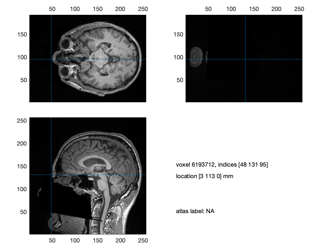
Figure: The location of the nasion indicated by the crosshair in the anatomical MRI image
Exercise 1
Inspect the location of the LPA and RPA.
Now, we can coregister the MRI image to the coordinate system as used for the MEG sensor positions:
cfg              = [];
cfg.method       = 'fiducial';
% this information has been obtained from the .json associated with the anatomical image
cfg.fiducial.nas = coordinates.AnatomicalLandmarkCoordinates.Nasion';
cfg.fiducial.lpa = coordinates.AnatomicalLandmarkCoordinates.LPA';
cfg.fiducial.rpa = coordinates.AnatomicalLandmarkCoordinates.RPA';
cfg.coordsys     = 'neuromag';
mri              = ft_volumerealign(cfg, mri_orig);

filename = fullfile(subj.outputpath, 'anatomy', subj.name, sprintf('%s_mri.mat', subj.name));
% save(filename, 'mri');
% load(filename, 'mri');
Exercise 2
Inspect the location of the NAS, LPA and RPA of the coregistered MRI. Pay special attention to the location coordinates, as compared to the location coordinates of the original MRI.
Following the initial alignment of the MRI with the MEG coordinate system on the basis of the anatomical landmarks, we can further improve the coregistration by using an interactive-closest-points (ICP) procedure. In that procedure, we fit the scalp surface than can be obtained from the MRI to a detailed measurement of the scalp surface using a Polhemus electromagnetic tracker. The measured head surface points can be read with ft_read_headshape and are available as sub-01/ses-meg/meg/sub-01_ses-meg_headshape.pos or can be read directly from the fif file.
Creation of the single shell head model
Now, to create a single-shell model of the inner surface of the skull, we need a segmentation of the MRI, which can be achieved with the function ft_volumesegment. This function uses SPM for segmentation, and by default returns a probabilistic segmentation of the grey, white and csd compartments. Here, we only need a description of the surface of the brain, which is obtained by combining the grey/white/csf and thresholding the image.
thr = 0.5;

% segment the coregistered mri
cfg                = [];
cfg.output         = 'brain';
cfg.brainthreshold = thr;
seg = ft_volumesegment(cfg, mri);

% create the mesh
cfg        = [];
cfg.method = 'singleshell';
headmodel  = ft_prepare_headmodel(cfg, seg);

filename = fullfile(subj.outputpath, 'anatomy', subj.name, sprintf('%s_headmodel.mat', subj.name));
% save(filename, 'headmodel');
% load(filename, 'headmodel');
You can now visualize the headmodel in combination with the anatomical image:
cfg = [];
cfg.intersectmesh = headmodel.bnd;
ft_sourceplot(cfg, mri);
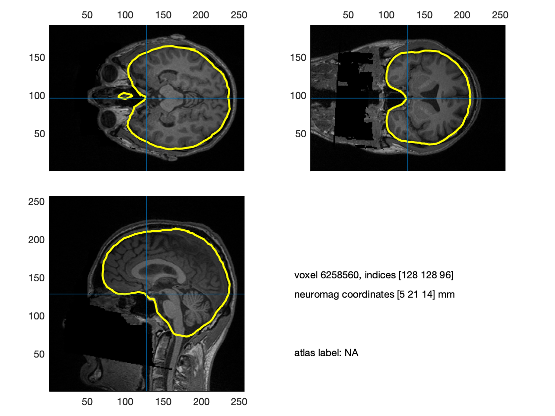
Figure: The headmodel visualized on top of the volumetric anatomical MRI
Creation of a source model based on the cortical sheet
To creation of a state-of-the-art source model based on the cortical sheet is described in a dedicated tutorial. Source reconstruction algorithms that assume distributed sources - for instance Minimum Norm Estimates (MNE) - really require these cortical models. For beamformers these are not absolutely necessary and you can also use a regular 3D grid.
The generation of a source model based on the cortical sheet can be rather time consuming, so we are not going to do that here. Instead, the sourcemodels have already been computed, according to a slightly modified version of the recipe described in the aforementioned tutorial. Below, the code is referenced that was used to generate the source models. It serves as an illustrative example, because it was executed on the Donders Institute’s compute cluster, which uses a specific way to execute computational jobs (qsub). The overall idea would be to tweak a set of shell scripts ft_freesurferscript.sh and ft_postfreesurferscript.sh that are located in fieldtrip/bin, and execute those on your own computer. This requires a Linux or macOS environment with FreeSurfer and HCP workbench installed.
In contrast to the source model tutorial that is written for CTF data, the input MRI image here coregistered to the Neuromag MEG coordinate system. This coordinate system is sufficiently similar to the coordinate system expected by freesurfer, so that the overall (post)freesurfer pipeline runs through fine. If, by contrast, the MEG coordinate system is according to the CTF system’s convention, an intermediate (temporary) coregistration is required.
% this part creates a FreeSurfer output base directory and fills it with
% an anatomical image that is going to be used by FreeSurfer

mkdir(fullfile(subj.outputpath, 'anatomy', subj.name, 'freesurfer'));
cfg              = [];
cfg.filename     = fullfile(subj.outputpath, 'anatomy', subj.name, 'freesurfer', subj.name);
cfg.filetype     = 'mgz'; % not sure whether this is supported in Windows
cfg.parameter    = 'anatomy';
ft_volumewrite(cfg, mri);

% this part runs a standard automatic FreeSurfer pipeline. It is not
% guaranteed to work out-of-the-box and may require some manual tweaks

[dum, ft_path] = ft_version;
scriptname = fullfile(ft_path,'bin','ft_freesurferscript.sh');
subj_dir   = fullfile(subj.outputpath, 'anatomy', subj.name, 'freesurfer');
cmd_str    = sprintf('echo "%s %s %s" | qsub -l walltime=20:00:00,mem=8gb -N sub-%02d', scriptname, subj_dir, subj.name, subj.id);
system(cmd_str);

% this part runs a set of postprocessing steps, and requires connectome workbench to be available

[dum, ft_path] = ft_version;
scriptname = fullfile(ft_path,'bin','ft_postfreesurferscript.sh');
subj_dir   = fullfile(subj.outputpath, 'anatomy', subj.name, 'freesurfer');
templ_dir  = '/home/megmethods/roboos/standard_mesh_atlases';
cmd_str    = sprintf('echo "%s %s %s %s" | qsub -l walltime=20:00:00,mem=8gb -N sub-%02d', scriptname, subj_dir, subj.name, templ_dir, subj.id);
system(cmd_str);
The result of the ft_freesurferscript.sh is a ‘standard’ set of FreeSurfer generated files, which in this case are stored in the freesurfer/sub-01 directory. Relevant for our subsequent endeavours are the files located in the freesurfer/sub-01/surf folder. Checking the content of such a surf folder, which can be done by typing:
ls
on the MATLAB command line, you see something like this:
>> ls
lh.area            lh.inflated         lh.smoothwm         lh.smoothwm.nofix  lh.white.preaparc.H  rh.defect_chull    rh.pial             rh.smoothwm.K2.crv  rh.white
lh.area.mid        lh.inflated.H       lh.smoothwm.BE.crv  lh.sphere          lh.white.preaparc.K  rh.defect_labels   rh.qsphere.nofix    rh.smoothwm.S.crv   rh.white.preaparc
lh.area.pial       lh.inflated.K       lh.smoothwm.C.crv   lh.sphere.reg      rh.area              rh.inflated        rh.smoothwm         rh.smoothwm.nofix   rh.white.preaparc.H
lh.avg_curv        lh.inflated.nofix   lh.smoothwm.FI.crv  lh.sulc            rh.area.mid          rh.inflated.H      rh.smoothwm.BE.crv  rh.sphere           rh.white.preaparc.K
lh.curv            lh.jacobian_white   lh.smoothwm.H.crv   lh.thickness       rh.area.pial         rh.inflated.K      rh.smoothwm.C.crv   rh.sphere.reg
lh.curv.pial       lh.orig             lh.smoothwm.K.crv   lh.volume          rh.avg_curv          rh.inflated.nofix  rh.smoothwm.FI.crv  rh.sulc
lh.defect_borders  lh.orig.nofix       lh.smoothwm.K1.crv  lh.w-g.pct.mgh     rh.curv              rh.jacobian_white  rh.smoothwm.H.crv   rh.thickness
lh.defect_chull    lh.pial             lh.smoothwm.K2.crv  lh.white           rh.curv.pial         rh.orig            rh.smoothwm.K.crv   rh.volume
lh.defect_labels   lh.qsphere.nofix    lh.smoothwm.S.crv   lh.white.preaparc  rh.defect_borders    rh.orig.nofix      rh.smoothwm.K1.crv  rh.w-g.pct.mgh
That is, a bunch of files, which exist in an ‘rh’ and ‘lh’ version. Each of the cortical hemispheres is represented in a separate file. We can load these surface based representations in FieldTrip, and visualize them in the following way:
pial = ft_read_headshape({'lh.pial' 'rh.pial'});
figure;
ft_plot_mesh(pial, 'vertexcolor', pial.sulc);
h1 = light('position',[-1 0 0]);
h2 = light('position',[1 0 0]);
material dull
lighting gouraud; set(gcf,'color','w');
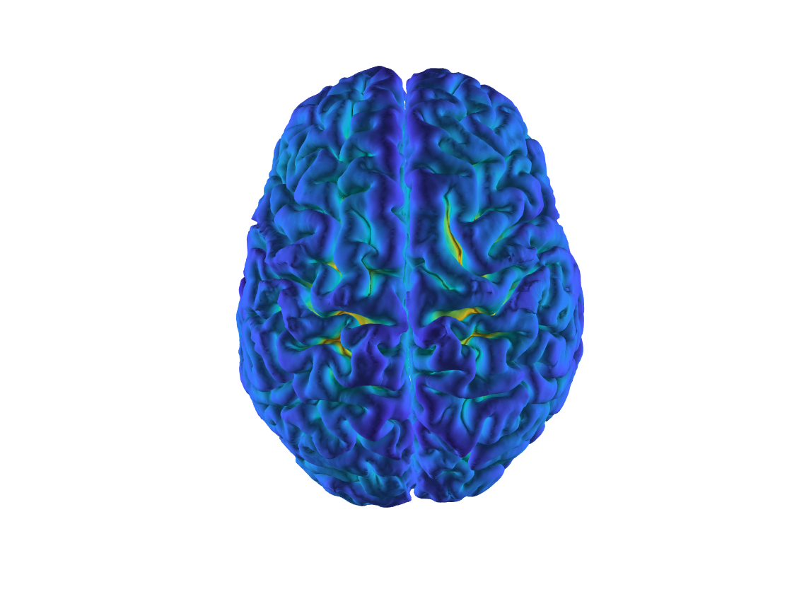
Figure: The pial surface extracted by freesurfer
Inspecting the variable ‘pial’, you will see something like this:
>> pial

pial =
struct with fields:
                pos: [259215x3 double]
                tri: [518422x3 double]
               sulc: [259215x1 double]
               curv: [259215x1 double]
               area: [259215x1 double]
          thickness: [259215x1 double]
     brainstructure: [259215x1 double]
brainstructurelabel: {2x1 cell}
The relevant topological information is represented in the pos and tri fields, where the 259215x3 pos-matrix contains a set of 3D coordinates of the vertices of a triangulated mesh, and the 518422x3 tri-matrix contains the indices of the vertices that make up the individual triangles. The 259215x1 vectors in the sulc/curv/area/thickness/brainstructure reflect scalar parameters at each of the vertices, corresponding to local properties of the cortical sheet.
For the purpose of MEG-based source reconstruction, the FreeSurfer surface needs to be downsampled a lower number of vertices, since the large number of vertices is just an overkill, given the limited spatial resolution of MEG. Moreover, each individual cortical sheet (and hemisphere) has a different number of vertex location, which makes it easy to combine these native cortical meshes across subjects. The ft_postfreesurferscript.sh does a surface-based registration to a template surface, reorganising the meshes to have a fixed number of ~164000 vertices per hemisphere, followed by a downsampling step, resulting in meshes that are topologically equivalent to the high resolution meshes, but with a lower number of vertices per hemisphere (~32k, ~8k, ~4k). The idea is now that each of the vertices of the resulting meshes (over subjects) are registered to a standardized template, so they can be easily compared across subjects, facilitating group level analysis later on.
The software needed for this step is connectome workbench. The output of this step is stored here in the freesurfer/workbench directory. Checking the content of such a workbench folder, you see something like this:
>> ls
fsaverage                                          sub-01.L.midthickness.164k_fs_LR.surf.gii    sub-01.L.white.8k_fs_LR.surf.gii                  sub-01.R.midthickness.8k_fs_LR.surf.gii
sub-01.164k_fs_LR.wb.spec                          sub-01.L.midthickness.32k_fs_LR.surf.gii     sub-01.L.white.native.surf.gii                    sub-01.R.midthickness.native.surf.gii
sub-01.32k_fs_LR.wb.spec                           sub-01.L.midthickness.4k_fs_LR.surf.gii      sub-01.R.ArealDistortion_FS.164k_fs_LR.shape.gii  sub-01.R.pial.164k_fs_LR.surf.gii
sub-01.4k_fs_LR.wb.spec                            sub-01.L.midthickness.8k_fs_LR.surf.gii      sub-01.R.ArealDistortion_FS.32k_fs_LR.shape.gii   sub-01.R.pial.32k_fs_LR.surf.gii
sub-01.8k_fs_LR.wb.spec                            sub-01.L.midthickness.native.surf.gii        sub-01.R.ArealDistortion_FS.4k_fs_LR.shape.gii    sub-01.R.pial.4k_fs_LR.surf.gii
sub-01.L.ArealDistortion_FS.164k_fs_LR.shape.gii   sub-01.L.pial.164k_fs_LR.surf.gii            sub-01.R.ArealDistortion_FS.8k_fs_LR.shape.gii    sub-01.R.pial.8k_fs_LR.surf.gii
sub-01.L.ArealDistortion_FS.32k_fs_LR.shape.gii    sub-01.L.pial.32k_fs_LR.surf.gii             sub-01.R.ArealDistortion_FS.native.shape.gii      sub-01.R.pial.native.surf.gii
sub-01.L.ArealDistortion_FS.4k_fs_LR.shape.gii     sub-01.L.pial.4k_fs_LR.surf.gii              sub-01.R.aparc.164k_fs_LR.label.gii               sub-01.R.refsulc.164k_fs_LR.shape.gii
sub-01.L.ArealDistortion_FS.8k_fs_LR.shape.gii     sub-01.L.pial.8k_fs_LR.surf.gii              sub-01.R.aparc.32k_fs_LR.label.gii                sub-01.R.roi.native.shape.gii
sub-01.L.ArealDistortion_FS.native.shape.gii       sub-01.L.pial.native.surf.gii                sub-01.R.aparc.4k_fs_LR.label.gii                 sub-01.R.sphere.164k_fs_LR.surf.gii
sub-01.L.aparc.164k_fs_LR.label.gii                sub-01.L.refsulc.164k_fs_LR.shape.gii        sub-01.R.aparc.8k_fs_LR.label.gii                 sub-01.R.sphere.32k_fs_LR.surf.gii
sub-01.L.aparc.32k_fs_LR.label.gii                 sub-01.L.roi.native.shape.gii                sub-01.R.aparc.a2009s.164k_fs_LR.label.gii        sub-01.R.sphere.4k_fs_LR.surf.gii
sub-01.L.aparc.4k_fs_LR.label.gii                  sub-01.L.sphere.164k_fs_LR.surf.gii          sub-01.R.aparc.a2009s.32k_fs_LR.label.gii         sub-01.R.sphere.8k_fs_LR.surf.gii
sub-01.L.aparc.8k_fs_LR.label.gii                  sub-01.L.sphere.32k_fs_LR.surf.gii           sub-01.R.aparc.a2009s.4k_fs_LR.label.gii          sub-01.R.sphere.native.surf.gii
sub-01.L.aparc.a2009s.164k_fs_LR.label.gii         sub-01.L.sphere.4k_fs_LR.surf.gii            sub-01.R.aparc.a2009s.8k_fs_LR.label.gii          sub-01.R.sphere.reg.native.surf.gii
sub-01.L.aparc.a2009s.32k_fs_LR.label.gii          sub-01.L.sphere.8k_fs_LR.surf.gii            sub-01.R.aparc.a2009s.native.label.gii            sub-01.R.sphere.reg.reg_LR.native.surf.gii
sub-01.L.aparc.a2009s.4k_fs_LR.label.gii           sub-01.L.sphere.native.surf.gii              sub-01.R.aparc.native.label.gii                   sub-01.R.sulc.164k_fs_LR.shape.gii
sub-01.L.aparc.a2009s.8k_fs_LR.label.gii           sub-01.L.sphere.reg.native.surf.gii          sub-01.R.atlasroi.164k_fs_LR.shape.gii            sub-01.R.sulc.32k_fs_LR.shape.gii
sub-01.L.aparc.a2009s.native.label.gii             sub-01.L.sphere.reg.reg_LR.native.surf.gii   sub-01.R.atlasroi.32k_fs_LR.shape.gii             sub-01.R.sulc.4k_fs_LR.shape.gii
sub-01.L.aparc.native.label.gii                    sub-01.L.sulc.164k_fs_LR.shape.gii           sub-01.R.atlasroi.4k_fs_LR.shape.gii              sub-01.R.sulc.8k_fs_LR.shape.gii
sub-01.L.atlasroi.164k_fs_LR.shape.gii             sub-01.L.sulc.32k_fs_LR.shape.gii            sub-01.R.atlasroi.8k_fs_LR.shape.gii              sub-01.R.sulc.native.shape.gii
sub-01.L.atlasroi.32k_fs_LR.shape.gii              sub-01.L.sulc.4k_fs_LR.shape.gii             sub-01.R.atlasroi.native.shape.gii                sub-01.R.thickness.164k_fs_LR.shape.gii
sub-01.L.atlasroi.4k_fs_LR.shape.gii               sub-01.L.sulc.8k_fs_LR.shape.gii             sub-01.R.curvature.164k_fs_LR.shape.gii           sub-01.R.thickness.32k_fs_LR.shape.gii
sub-01.L.atlasroi.8k_fs_LR.shape.gii               sub-01.L.sulc.native.shape.gii               sub-01.R.curvature.32k_fs_LR.shape.gii            sub-01.R.thickness.4k_fs_LR.shape.gii
sub-01.L.atlasroi.native.shape.gii                 sub-01.L.thickness.164k_fs_LR.shape.gii      sub-01.R.curvature.4k_fs_LR.shape.gii             sub-01.R.thickness.8k_fs_LR.shape.gii
sub-01.L.curvature.164k_fs_LR.shape.gii            sub-01.L.thickness.32k_fs_LR.shape.gii       sub-01.R.curvature.8k_fs_LR.shape.gii             sub-01.R.thickness.native.shape.gii
sub-01.L.curvature.32k_fs_LR.shape.gii             sub-01.L.thickness.4k_fs_LR.shape.gii        sub-01.R.curvature.native.shape.gii               sub-01.R.very_inflated.164k_fs_LR.surf.gii
sub-01.L.curvature.4k_fs_LR.shape.gii              sub-01.L.thickness.8k_fs_LR.shape.gii        sub-01.R.flat.164k_fs_LR.surf.gii                 sub-01.R.very_inflated.32k_fs_LR.surf.gii
sub-01.L.curvature.8k_fs_LR.shape.gii              sub-01.L.thickness.native.shape.gii          sub-01.R.flat.32k_fs_LR.surf.gii                  sub-01.R.very_inflated.4k_fs_LR.surf.gii
sub-01.L.curvature.native.shape.gii                sub-01.L.very_inflated.164k_fs_LR.surf.gii   sub-01.R.inflated.164k_fs_LR.surf.gii             sub-01.R.very_inflated.8k_fs_LR.surf.gii
sub-01.L.flat.164k_fs_LR.surf.gii                  sub-01.L.very_inflated.32k_fs_LR.surf.gii    sub-01.R.inflated.32k_fs_LR.surf.gii              sub-01.R.very_inflated.native.surf.gii
sub-01.L.flat.32k_fs_LR.surf.gii                   sub-01.L.very_inflated.4k_fs_LR.surf.gii     sub-01.R.inflated.4k_fs_LR.surf.gii               sub-01.R.white.164k_fs_LR.surf.gii
sub-01.L.inflated.164k_fs_LR.surf.gii              sub-01.L.very_inflated.8k_fs_LR.surf.gii     sub-01.R.inflated.8k_fs_LR.surf.gii               sub-01.R.white.32k_fs_LR.surf.gii
sub-01.L.inflated.32k_fs_LR.surf.gii               sub-01.L.very_inflated.native.surf.gii       sub-01.R.inflated.native.surf.gii                 sub-01.R.white.4k_fs_LR.surf.gii
sub-01.L.inflated.4k_fs_LR.surf.gii                sub-01.L.white.164k_fs_LR.surf.gii           sub-01.R.midthickness.164k_fs_LR.surf.gii         sub-01.R.white.8k_fs_LR.surf.gii
sub-01.L.inflated.8k_fs_LR.surf.gii                sub-01.L.white.32k_fs_LR.surf.gii            sub-01.R.midthickness.32k_fs_LR.surf.gii          sub-01.R.white.native.surf.gii
sub-01.L.inflated.native.surf.gii                  sub-01.L.white.4k_fs_LR.surf.gii             sub-01.R.midthickness.4k_fs_LR.surf.gii           sub-01.native.wb.spec
The important thing to note is that the majority of files with the .gii extension are gifti files, rather than the legacy fileformat used by FreeSurfer. Gifti files are versatile and represent geometric data defined as tessellated meshes. Next to a specific naming scheme of the files, connectome workbench uses a specific file naming convention for representing the different types of data. Let’s dissect the file naming in some detail:
<subjectname>.<hemisphere>.<somename>.<number>k_fs_LR.<someothername>.gii
Starting off with
Next to the surf.gii files, there are shape.gii and label.gii files, which contain scalar information about local properties (for instance curvature) or contain parcellation information (for instance the anatomical parcel to which a given vertex belongs).
We can have a look at some files in a bit more detail:
wb_dir = fullfile(subj.outputpath, 'anatomy', subj.name, 'freesurfer', subj.name, 'workbench');
cd(wb_dir)

white         = ft_read_headshape('sub-01.L.white.8k_fs_LR.surf.gii');
midthickness  = ft_read_headshape('sub-01.L.midthickness.8k_fs_LR.surf.gii');
pial          = ft_read_headshape('sub-01.L.pial.8k_fs_LR.surf.gii');
inflated      = ft_read_headshape('sub-01.L.inflated.8k_fs_LR.surf.gii');
very_inflated = ft_read_headshape('sub-01.L.very_inflated.8k_fs_LR.surf.gii');
sphere        = ft_read_headshape('sub-01.L.sphere.8k_fs_LR.surf.gii');

figure;
h1 = subplot(2,3,1); ft_plot_mesh(white,'vertexcolor',white.thickness); lighting gouraud; material dull;light
h2 = subplot(2,3,2); ft_plot_mesh(midthickness,'vertexcolor',white.thickness); lighting gouraud; material dull;light
h3 = subplot(2,3,3); ft_plot_mesh(pial,'vertexcolor',white.thickness); lighting gouraud; material dull;light
h4 = subplot(2,3,4); ft_plot_mesh(inflated,'vertexcolor',white.thickness); lighting gouraud; material dull;light
h5 = subplot(2,3,5); ft_plot_mesh(very_inflated,'vertexcolor',white.thickness); lighting gouraud; material dull;light
h6 = subplot(2,3,6); ft_plot_mesh(sphere,'vertexcolor',white.thickness); lighting gouraud; material dull;light
linkprop([h1 h2 h3 h4 h5 h6],'cameraposition');
The line with linkprop allows for simultaneous rotation of all objects, when switching on the rotate3d option in the figure. Click on the “rotate” symbol and use your mouse to look at the surfaces from all sides.
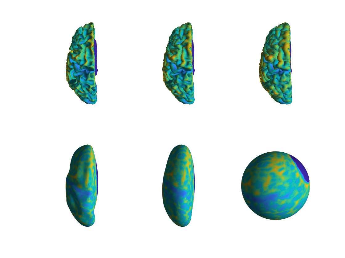
Figure: The different surfaces generated by connectome workbench
We now create a source model and save it to a .mat file to be readily available when performing source reconstruction later on.
wb_dir = fullfile(subj.outputpath, 'anatomy', subj.name, 'freesurfer', subj.name, 'workbench');
filename = fullfile(wb_dir, sprintf('%s.L.midthickness.8k_fs_LR.surf.gii.mat', subj.name));
sourcemodel = ft_read_headshape({filename strrep(filename, '.L.', '.R.')});
sourcemodel = ft_determine_units(sourcemodel);
sourcemodel.coordsys = 'neuromag';

filename = fullfile(subj.outputpath, 'anatomy', subj.name, sprintf('%s_sourcemodel.mat', subj.name));
% save(filename, 'sourcemodel');
% load(filename, 'sourcemodel');
Importantly, before proceeding any further, we want to check whether the headmodel and sourcemodel are nicely aligned to each other and to the sensor array:
subj = datainfo_subject(1);
hdr  = ft_read_header(subj.megfile{1}, 'coilaccuracy', 0);
grad = ft_convert_units(hdr.grad, 'mm');

load(fullfile(subj.outputpath, 'anatomy', subj.name, sprintf('%s_headmodel.mat', subj.name)));
load(fullfile(subj.outputpath, 'anatomy', subj.name, sprintf('%s_sourcemodel.mat', subj.name)));
headmodel   = ft_convert_units(headmodel,   'mm');
sourcemodel = ft_convert_units(sourcemodel, 'mm');

figure;hold on;
ft_plot_mesh(sourcemodel, 'facecolor', [0.8 0.2 0.2]);
ft_plot_headmodel(headmodel, 'edgecolor', 'none', 'facealpha', 0.3);
ft_plot_sens(grad);
h = light; lighting gouraud; material dull;
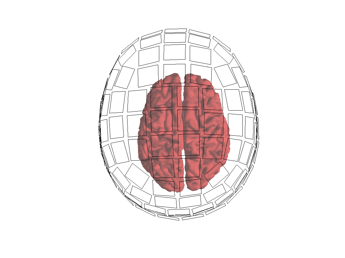
Figure: Coregistration between headmodel, sourcemodel and sensors