workshop / practicalmeeg2022 / handson_raw2erp /
Preprocessing raw data and computing ERPs/ERFs
This tutorial was written specifically for the PracticalMEEG workshop in Aix-en-Provence in December 2022 and is part of a coherent sequence of tutorials. It is an updated version of the corresponding tutorial for Paris 2019.
Introduction
In this tutorial, we will learn how to read in ‘raw’ data from a file, and to apply some basic processing and averaging in order to inspect event-related fields.
This tutorial only briefly covers the steps required to import data into FieldTrip and preprocess it. Rather, this tutorial has a focus on processing multiple runs of the same dataset, and exploring the different channel types. Preprocessing is covered in more detail in the preprocessing tutorial, which you can refer to if you want more details.
Preliminaries, definition of subject specific filenames, and definition of epochs-of-interest
Preprocessing of MEG/EEG data refers to the reading of the data, segmenting the data around interesting events such as triggers, temporal filtering and (optionally for EEG) rereferencing. The ft_preprocessing function takes care of all these steps, i.e., it reads the data and applies the preprocessing options.
There are two alternative approaches for preprocessing, which differ in the amount of memory required. The first approach is to read all data from the file into memory, apply filters, and subsequently cut the data into interesting segments. The second approach is to first identify the interesting segments, read those segments from the data file (possibly with some data padding) and apply the filters to those segments only. The remainder of this tutorial explains the second approach, as that is the most appropriate for large data sets such as the MEG data used in this tutorial. The approach for reading and filtering continuous data and segmenting afterwards is explained elsewhere.
Preprocessing involves several steps including defining epochs-of-interest from the dataset, filtering and artifact rejections. This tutorial covers how to identify epochs based on the recorded events during the experiment. Typically, this requires the use of ft_definetrial. For more details, see the preprocessing tutorial.
The output of ft_definetrial is a configuration structure containing the field cfg.trl. This is a matrix representing the relevant parts of the raw datafile which are to be selected for further processing. Each row in the trl matrix represents a single epoch-of-interest, and the trl matrix has at least 3 columns. The first column defines (in samples) the begin of each epoch with respect to how the data are stored in the raw datafile. The second column defines (in samples) the end of each epoch, and the third column specifies the offset (in samples) of the first sample within each epoch with respect to timepoint 0 within that epoch.
In this tutorial, the data is contained in 6 different fif files, one for every run. We will identify the segments for each file/run and subsequently read and preprocess each file/run.
First, to get started, we need to know which files to use. One way to do this, is to work with a subject specific text file that contains this information. Alternatively, in MATLAB, we can represent this information in a subject-specific data structure, where the fields contain the filenames of the files (including the directory) that are relevant. Here, we use the latter strategy.
We use the datainfo_subject function, which is provided in the code folder associated with this workshop. If we do the following:
subj = datainfo_subject(1);
We obtain a structure that looks like this:
 subj =
 struct with fields:
             id: 1
           name: 'sub-01'
        mrifile: '/Volumes/SamsungT3/practicalmeeg2022/ds000117-pruned/sub-01/ses-mri/anat/sub-01_ses-mri_acq-mprage_T1w.nii.gz'
        fidfile: '/Volumes/SamsungT3/practicalmeeg2022/ds000117-pruned/sub-01/ses-mri/anat/sub-01_ses-mri_acq-mprage_T1w.json'
     outputpath: '/Volumes/SamsungT3/practicalmeeg2022/derivatives'
        megfile: {6x1 cell}
     eventsfile: {6x1 cell}
We can now run the following chunk of code:
subj.trl = cell(6,1);
for run_nr = 1:6

  cfg = [];
  cfg.dataset = subj.megfile{run_nr};
  cfg.readbids = 'no'; % it looks like BIDS, but is not complete

  % this is what we can see in the BIDS events.tsv file
  Famous      = [5 6 7];
  Unfamiliar  = [13 14 15];
  Scrambled   = [17 18 19];

  cfg.trialfun = 'ft_trialfun_general';
  cfg.trialdef.eventtype = 'STI101';
  cfg.trialdef.eventvalue = [Famous Unfamiliar Scrambled];
  cfg.trialdef.prestim = 0.5;
  cfg.trialdef.poststim = 1.2;

  cfg = ft_definetrial(cfg);

  % remember the trial definition for each run
  subj.trl{run_nr} = cfg.trl;

end % for each run
In the previous code we are making use of numeric trigger codes instead of the events that are coded in the BIDS dataset. This is because the pruned derivative dataset is NOT according to the BIDS standard. First of all, some files are missing due to the pruning. More importantly, MEG and EEG derivatives are not finalized and not part of BIDS yet. They are being discussed here.
Although we have the MaxFiltered fif file with the data and original trigger codes
sub-01_ses-meg_task-facerecognition_run-01_proc-sss_meg.fif
according to BIDS we would also have expected its sidecars, but these are missing:
sub-01_ses-meg_task-facerecognition_run-01_proc-sss_meg.json
sub-01_ses-meg_task-facerecognition_run-01_proc-sss_events.tsv
Reading in raw data from disk
In the section above, we have created a set of trl matrices, which contain, for each of the runs in the experiment, a specification of the begin, and endpoint of the relevant epochs. We can now proceed with reading in the data, applying a bandpass filter, and excluding filter edge effects in the data-of-interest, by using the cfg.padding argument. The below chunk of code takes some time (and RAM) to compute, so if your computer is not up to this, you can also skip this step, and load in the sub-01_data.mat from the derivatives/raw2erp/sub-01 folder:
rundata = cell(1,6);
for run_nr = 1:6

  cfg         = [];
  cfg.dataset = subj.megfile{run_nr};
  cfg.trl     = subj.trl{run_nr};

  % MEG specific settings
  cfg.channel = 'MEG';
  cfg.demean  = 'yes';
  cfg.coilaccuracy = 0;
  cfg.bpfilter = 'yes';
  cfg.bpfilttype = 'firws';
  cfg.bpfreq  = [1 40];
  cfg.padding = 3;
  data_meg    = ft_preprocessing(cfg);

  % EEG specific settings
  cfg.channel    = {'EEG' '-EEG061' '-EEG062' '-EEG063' '-EEG064'}; % exclude EOG/ECG/etc hard coded assumed to be this list
  cfg.demean     = 'yes';
  cfg.reref      = 'yes';
  cfg.refchannel = 'all'; % average reference
  data_eeg       = ft_preprocessing(cfg);

  % this is what we can see in the BIDS channels.tsv file
  % EEG061    HEOG    V    horizontaleog
  % EEG062    VEOG    V    verticaleog
  % EEG063    ECG     V    cardiac

  % settings for EOG and ECG channels
  cfg.channel = {'EEG061' 'EEG062' 'EEG063'};
  cfg.demean  = 'yes';
  cfg.reref   = 'no';
  cfg.bpfilter = 'no';

  % use a one-to-one montage to rename the channels, see FT_APPLY_MONTAGE
  cfg.montage.labelold = {'EEG061' 'EEG062' 'EEG063'};
  cfg.montage.labelnew = {'HEOG' 'VEOG' 'ECG'};
  cfg.montage.tra      = eye(3);
  data_exg    = ft_preprocessing(cfg);

  % settings for all other channels
  cfg.channel = {'all', '-MEG', '-EEG'};
  cfg.montage = []; % remove the previously applied montage
  cfg.demean  = 'no';
  cfg.reref   = 'no';
  cfg.bpfilter = 'no';
  data_other  = ft_preprocessing(cfg);

  cfg            = [];
  cfg.resamplefs = 300;
  data_meg       = ft_resampledata(cfg, data_meg);
  data_eeg       = ft_resampledata(cfg, data_eeg);
  data_exg       = ft_resampledata(cfg, data_exg);
  data_other     = ft_resampledata(cfg, data_other);

  % append the different channel sets into a single structure
  rundata{run_nr} = ft_appenddata([], data_meg, data_eeg, data_exg, data_other);
  clear data_meg data_eeg data_exg data_other
end % for each run

data = ft_appenddata([], rundata{:});
clear rundata;

% we could save it to disk, or when skipping the code above we can read it from disk
filename = fullfile(subj.outputpath, 'raw2erp', subj.name, sprintf('%s_data.mat', subj.name));
% save(filename, 'data');
% load(filename, 'data');
The above chunk of code uses ft_preprocessing four times per run, with channel type specific processing options. Note the exclusion of a subset of the EEG channels which correspond to non-brain recording EEG signals (EOG/ECG etc.). The EEG data are average-referenced, the other channels are not. After the data for each group of channels has been read from disk, ft_resampledata is used to downsample the data to a sampling frequency of 300 Hz. Then, the data structures are combined into a single run-specific data structure, using ft_appenddata.
There is no advantage in resampling the data other than saving some memory. If your computer is big enough to handle your data, we recommend not to resample as there can be some annoying side effects. The anti-aliasing filter can affect your data, and post-hoc bookeeping of events (which are indicated with sample numbers) gets more complicated.
In this specific case we are resampling to fit it in memory of the participants’ laptops and to speed up subsequent computations.
The recorded data apparently has a delay of 34.5 ms relative to the onset of the triggers and relative to the events.tsv file. This can be corrected with ft_redefinetrial like this
cfg            = [];
cfg.offset     = -0.0345 * data.fsample; % expressed in samples
data_corrected = ft_redefinetrial(cfg, data);
In the remainder we will continue with the uncorrected data, as that was used for the processing of all 16 subjects’ source reconstructed results that we will use for group-level statistics. So please keep in mind that the time axis is off by 34.5 ms.
Compute condition-specific averages (ERFs/ERPs)
Once the data has been epoched and filtered, we can proceed with computing event-related averages, which are called ERFs for MEG and ERPs for EEG. This is achieved with ft_timelockanalysis. In order to selectively average across epochs from different conditions, we make use of the data.trialinfo field, which contains a numeric indicator of the condition to which that particular epoch belongs. Thus, we can do:
cfg        = [];
cfg.preproc.demean = 'yes';
cfg.preproc.baselinewindow = [-0.1 0];

% this is what we can see in the BIDS events.tsv file
Famous      = [5 6 7];
Unfamiliar  = [13 14 15];
Scrambled   = [17 18 19];

cfg.trials = ismember(data.trialinfo(:,1), Famous);
avg_famous = ft_timelockanalysis(cfg, data);

cfg.trials = ismember(data.trialinfo(:,1), Unfamiliar);
avg_unfamiliar = ft_timelockanalysis(cfg, data);

cfg.trials = ismember(data.trialinfo(:,1), Scrambled);
avg_scrambled = ft_timelockanalysis(cfg, data);

cfg.trials = ismember(data.trialinfo(:,1), [Famous Unfamiliar]);
avg_faces  = ft_timelockanalysis(cfg, data);

filename = fullfile(subj.outputpath, 'raw2erp', subj.name, sprintf('%s_timelock.mat', subj.name));
% save(filename, 'avg_famous', 'avg_unfamiliar', 'avg_scrambled', 'avg_faces');
% load(filename, 'avg_famous', 'avg_unfamiliar', 'avg_scrambled', 'avg_faces');
Visualisation of the ERFs
At this stage, we have a set of spatiotemporal matrices, reflecting the electrophysiological response to different types of stimuli. In order to visualize the time courses, and interpret the spatial distribution of the responses, we can use a combination of the following FieldTrip functions: ft_multiplotER, ft_topoplotER, ft_singleplotER. With the exception of ft_singleplotER these functions require a specification of (a 2D projection) of the positions of the sensors/electrodes. In FieldTrip, this is specified by the cfg.layout option; you can read more about this in the layout tutorial. More information about the visualisation of sensor (and source) level data can be found in the plotting tutorial.
First of all, let’s look at the plotting the data directly using standard MATLAB plotting commands. If we look at one of the averaged ERP/ERF data structures, we can recognize the field time, avg and label.
>> disp(avg_famous)
      grad: [1x1 struct]
      elec: [1x1 struct]
      time: [-0.4988 -0.4955 -0.4921 -0.4888 -0.4855 -0.4821 -0.4788  … ]
     label: {403x1 cell}
       avg: [403x510 double]
       var: [403x510 double]
       dof: [403x510 double]
    dimord: 'chan_time'
       cfg: [1x1 struct]
To find a specific channel, we can use the following
find(strcmp(avg_famous.label, 'EEG065'))
and to plot the ‘EEG065’ channel channel we can do
plot(avg_famous.time, avg_famous.avg(367,:), 'b')
hold on
plot(avg_unfamiliar.time, avg_unfamiliar.avg(367,:), 'r')
plot(avg_scrambled.time, avg_scrambled.avg(367,:), 'g')
The same figure can be achieved using the following code
cfg = [];
cfg.channel = 'EEG065'
ft_singleplotER(cfg, avg_famous, avg_unfamiliar, avg_scrambled)
There are in total 102 magnetometer channels, 204 planar gradiometer channels, and 70 EEG channels. We would not want to make a separate figure for each of them. We can plot the channels of one specific type (and with the same units) together in one figure, where each channel is plotted at the corresponding location.
% visualize the magnetometer data
cfg        = [];
cfg.layout = 'neuromag306mag_helmet.mat';
figure; ft_multiplotER(cfg, avg_famous, avg_unfamiliar, avg_scrambled);
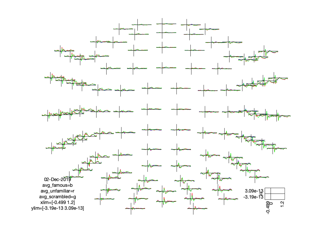
Figure: Distribution of magnetometer ERFs on a 2D projected sensory layout.
The figure that is generated by ft_multiplotER shows in a spatial distribution the ERFs on the different channels (in this case: magnetometers). The figure is interactive, and you can select subsets of channels by drawing a rectangle in the figure panel, followed by a left mouse click. This results in a figure that shows the condition specific ERFs as an average across the selected sensors. This representation is the same as when using ft_singleplotER. Selecting a time range in this figure results in a set of condition specific figures that show the topographical distribution of the ERF amplitude, as an average across the selected latency window.
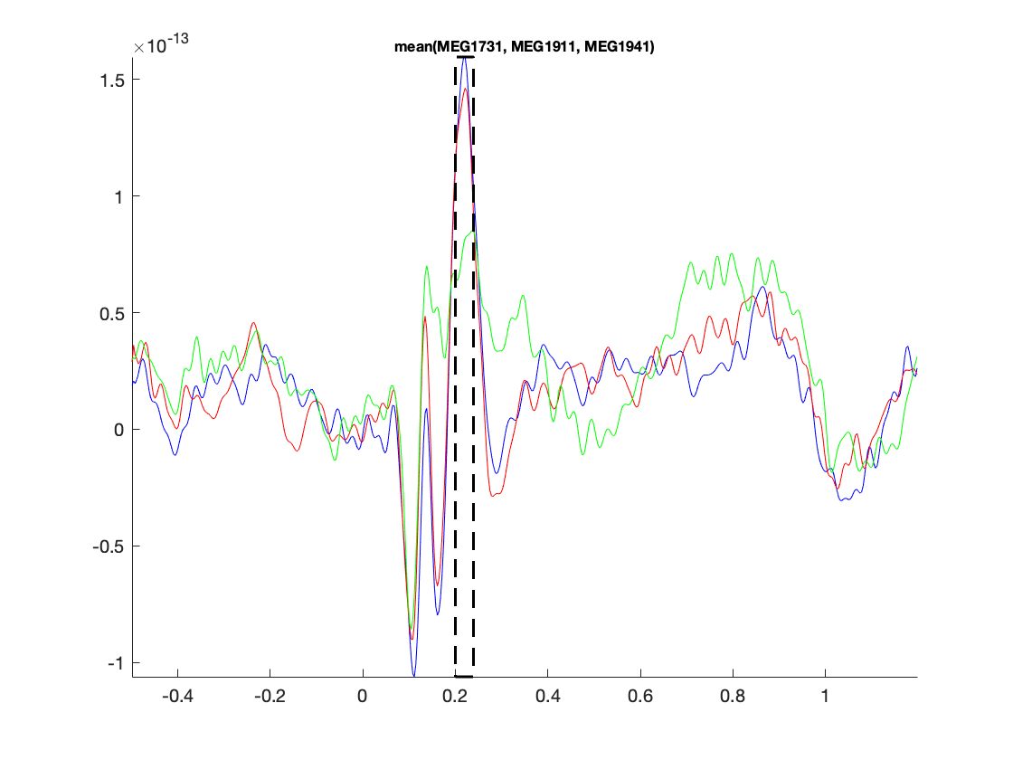
Figure: Average across selected magnetometers for each of the conditions.
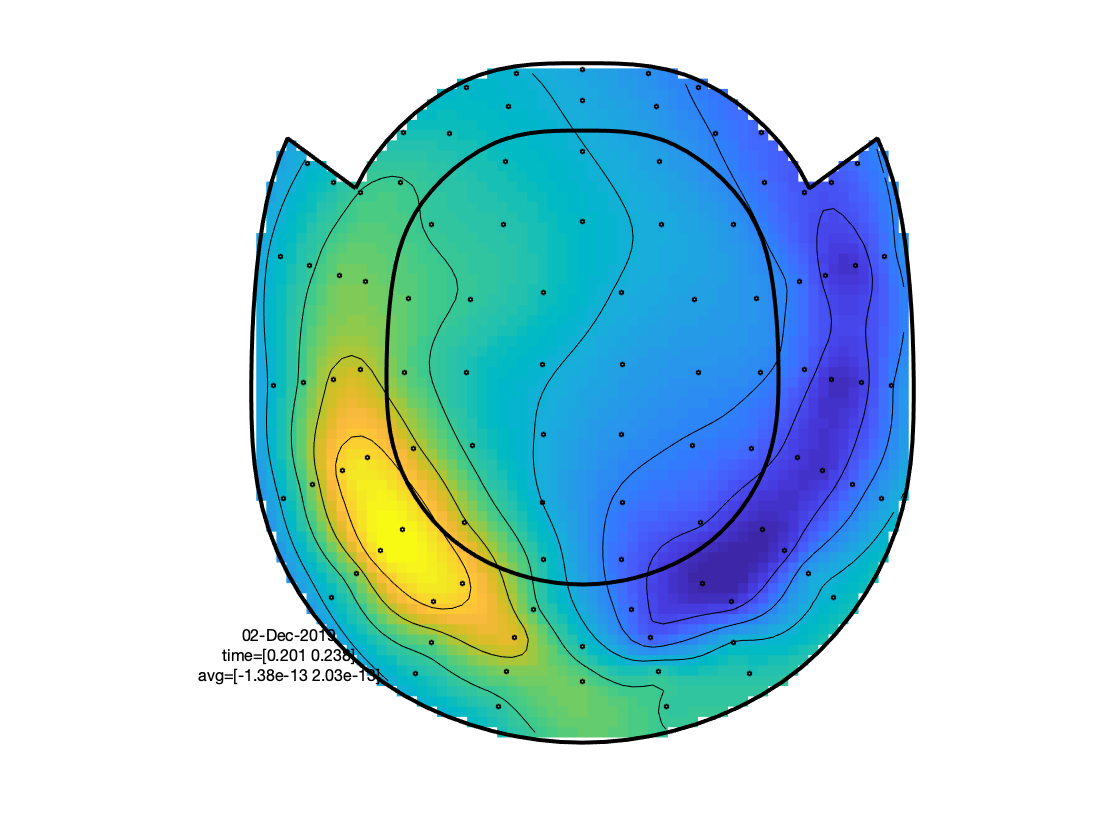
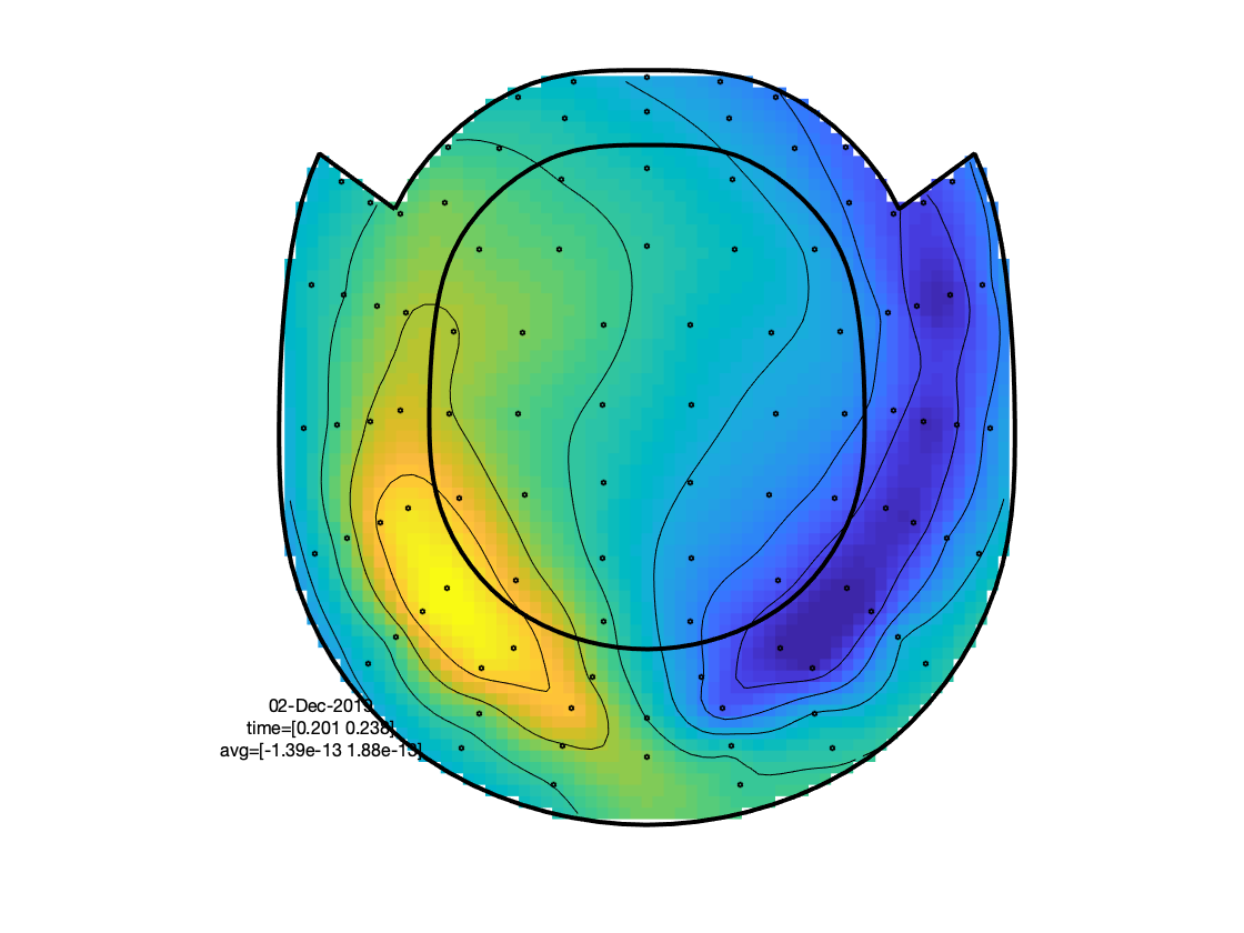
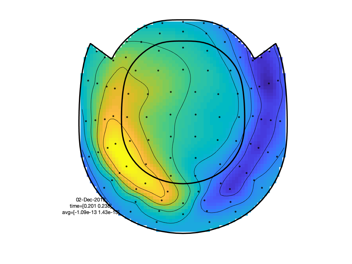
Figure: Topographies of average across selected latency window for each of the conditions.
For the visualisation of the gradiometers, we first compute the magnitude of the gradient by combining the ‘horizontal’ and ‘vertical’ gradients at each sensor location, using ft_combineplanar.
% combine planar gradients and visualize the gradiometer data
cfg              = [];
avg_faces_c      = ft_combineplanar(cfg, avg_faces);
avg_famous_c     = ft_combineplanar(cfg, avg_famous);
avg_unfamiliar_c = ft_combineplanar(cfg, avg_unfamiliar);
avg_scrambled_c  = ft_combineplanar(cfg, avg_scrambled);

cfg        = [];
cfg.layout = 'neuromag306cmb_helmet.mat';
figure; ft_multiplotER(cfg, avg_famous_c, avg_unfamiliar_c, avg_scrambled_c);
Just like plotting the MEG data, we can plot the EEG data. Since EEG data is recorded with widely different EEG systems, numbers of channels, and electrode layouts, we need to specify the layout of the channels to be plotted. This is explained in detail in the layout tutorial. FieldTrip also comes with a wide range of template layouts, but the 70-channel EEG system used here is not one of them. Luckily we have the electrode positions, which were digitized with a Polhemus.
% create an EEG channel layout on-the-fly and visualize the eeg data
cfg      = [];
cfg.elec = avg_faces.elec;
layout_eeg = ft_prepare_layout(cfg);

cfg        = [];
cfg.layout = layout_eeg;
figure; ft_multiplotER(cfg, avg_famous, avg_unfamiliar, avg_scrambled);
It is possible to visualize the data of the different channel types within a single figure. This leverages the interactive functionality of the figures and allows for easier comparison of latency-specific topographies. This can be achieved by first creating a combined layout with ft_appendlayout. This requires some handcrafting to the scaling of the EEG-based layout in relation to the MEG layouts.
When actually plotting the data with ft_multiplotER we need to specify a channel type specific scaling factor, to accommodate the different order of magnitude of the physical units in which the data are expressed. Alternatively, these scaling difference can be removed by application of a relative baseline (e.g., expressing the signals’ magnitude in dB relative to a specified baseline window), or by appropriately whitening the signals. Note, that the scaling factors here were obtained by eyeballing the data and do not represent ‘official’ scaling values.
cfg        = [];
cfg.layout = 'neuromag306mag_helmet.mat'; % magnetometers
layout_mag = ft_prepare_layout(cfg);

cfg        = [];
cfg.layout = 'neuromag306cmb_helmet.mat'; % combined planar gradiometers
layout_cmb = ft_prepare_layout(cfg);

% in order for this to work, the positions should be in the same order of magnitude
shiftval = min(layout_eeg.pos(1:70,:),[],1);
layout_eeg.pos = layout_eeg.pos - repmat(shiftval, numel(layout_eeg.label), 1);
layout_eeg.mask{1} = layout_eeg.mask{1} - repmat(shiftval, size(layout_eeg.mask{1},1), 1);
for k = 1:numel(layout_eeg.outline)
  layout_eeg.outline{k} = layout_eeg.outline{k} - repmat(shiftval, size(layout_eeg.outline{k},1), 1);
end

scaleval = max(layout_eeg.pos(1:70,:),[],1)./500;
layout_eeg.pos = layout_eeg.pos ./ repmat(scaleval, numel(layout_eeg.label), 1);
layout_eeg.mask{1} = layout_eeg.mask{1} ./ repmat(scaleval, size(layout_eeg.mask{1},1), 1);
for k = 1:numel(layout_eeg.outline)
  layout_eeg.outline{k} = layout_eeg.outline{k} ./ repmat(scaleval, size(layout_eeg.outline{k},1), 1);
end

layout_eeg.width(:)  = 64;
layout_eeg.height(:) = 48;

cfg = [];
cfg.distance = 180;
layout = ft_appendlayout(cfg, ft_appendlayout([], layout_mag, layout_cmb), layout_eeg);
You can use ft_plot_layout to inspect the layout that you have just constructed. See also the layout tutorial.
Now that we have a combined layout, we can plot all three datatypes and all three conditions at once. In the figure, you can make a selection to get a topoplot.
cfg = [];
cfg.layout    = layout;
cfg.gridscale = 150;
cfg.magscale  = 0.25e14;
cfg.gradscale = 1e12;
cfg.eegscale  = 1e6;
figure; ft_multiplotER(cfg, avg_famous_c, avg_unfamiliar_c, avg_scrambled_c);
Exercise 1
Explore the data, using the interactive property of the figure. Visualize the topographies of the ERF/ERPs in the latency window between 175 and 250 ms. Also inspect the topographies in the latency window from 300-450 ms. Explain the differences in topography (between latencies and channel types) based on putative underlying neuronal generators.
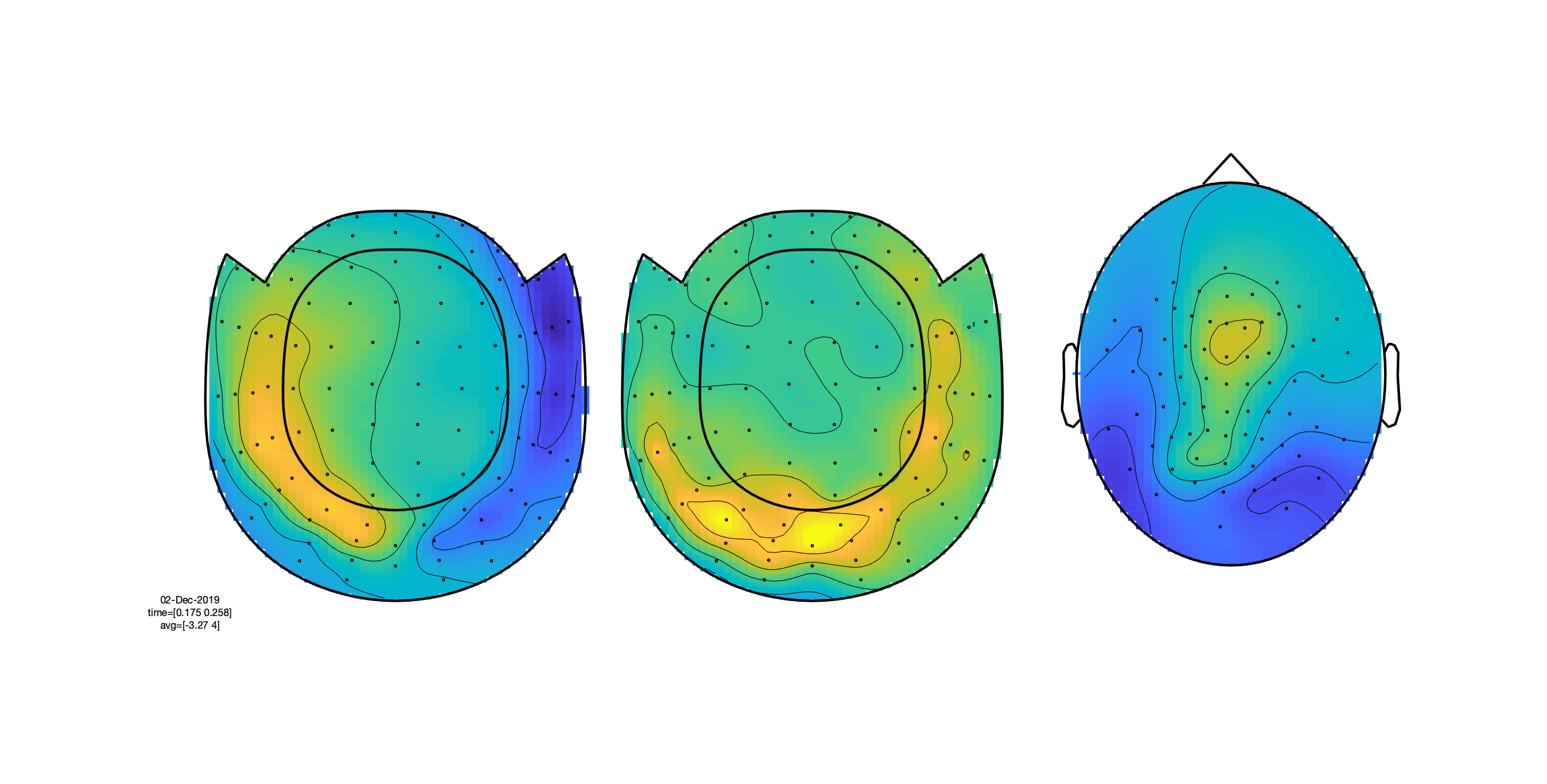
Figure: Topographies of the average across selected latency window for one of the conditions.
Exercise 2
The avg_famous structure not only contains the average, but also the variance. That can be used to compute the standard deviation and the standard error of the mean (SEM).
Use the following code to compute and plot the ERP together with the standard deviation:
avg          = avg_famous.avg(367,:);
avg_plus_sd  = avg + sqrt(avg_famous.var(367,:));
avg_minus_sd = avg - sqrt(avg_famous.var(367,:));

figure
plot(avg_famous.time, avg, 'b')
hold on
plot(avg_famous.time, avg_plus_sd, 'b:')
plot(avg_famous.time, avg_minus_sd, 'b:')
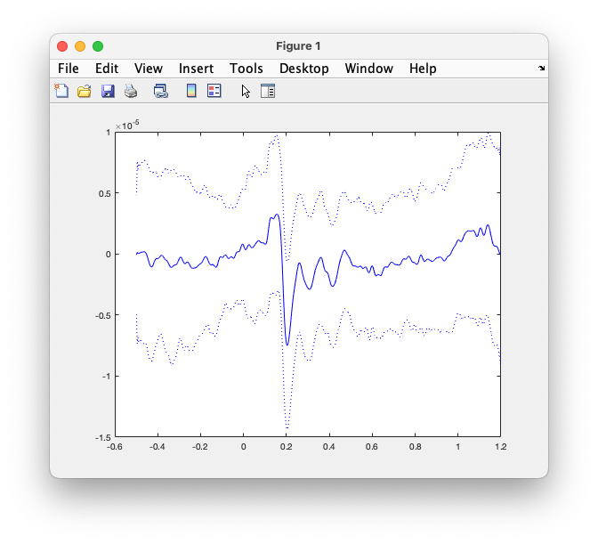
Figure: the averaged ERP on EEG065, plus and minus the standard deviation.
The standard deviation is quite large, among others because we have not yet performed any artifact correction. However, the average is rather clean due to it being computed over many trials. Use the following code to compute and plot the ERP together with the SD:
% there are 295 trials in this condition
avg_plus_sem  = avg + sqrt(avg_famous.var(367,:)) ./ sqrt(avg_famous.dof(367,:));
avg_minus_sem = avg - sqrt(avg_famous.var(367,:)) ./ sqrt(avg_famous.dof(367,:));

figure
plot(avg_famous.time, avg, 'b')
hold on
plot(avg_famous.time, avg_plus_sem, 'b:')
plot(avg_famous.time, avg_minus_sem, 'b:')
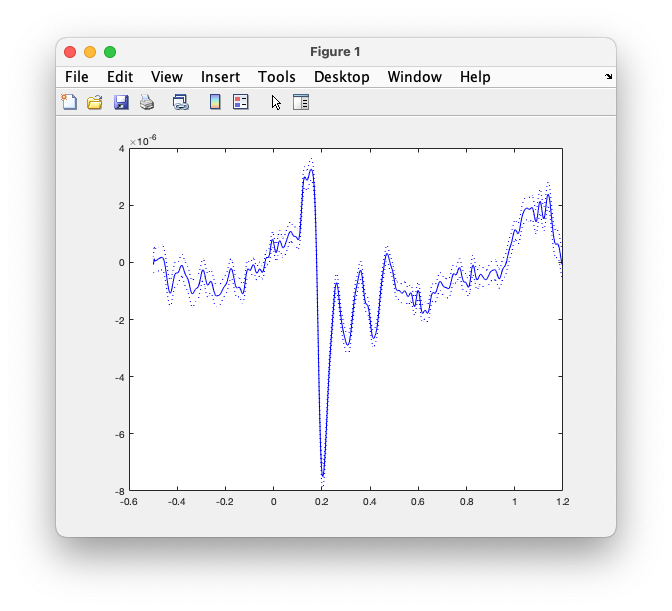
Figure: the averaged ERP on EEG065, plus and minus the SEM.
Exercise 3
Using the more low-level function ft_plot_vector we can make a more fancy visualisation of the confidence interval around the ERP. Try the following:
figure
ft_plot_vector(avg_famous.time, [avg_plus_sem; avg_minus_sem], 'highlightstyle', 'difference')
ft_plot_vector(avg_famous.time, avg, 'color', 'k', 'linewidth', 2)
axis tight
grid on
You can thresholded the ERP using the SEM to highlight parts of the time series:
significant = abs(avg) > 2*sqrt(avg_famous.var(367,:))./sqrt(avg_famous.dof(367,:));

figure
ft_plot_vector(avg_famous.time, avg, 'highlight', significant, 'highlightstyle', 'thickness', 'color', 'b');
axis tight
grid on
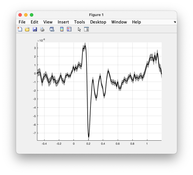
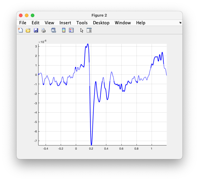
Figure: the ERP with the SEM as highlighted region, and the ERP that highlights the threshold.
Exercise 4
Rather than looking at the average and go to the thresholded statistics straight away, we can also look at the individual trials. For that it helps to represent the data according to the timelock structure, but keeping all the trials.
cfg = [];;
cfg.keeptrials = 'yes';
avg_trials = ft_timelockanalysis(cfg, data);
This results in the data being represented in a 3D array that is trials by channels by time: the dimord is rpt_chan_time. We can look at the time-locked response over all trials in a single channe; this is often called an ERP image.
figure
subplot(2,1,1); imagesc(squeeze(avg_all.trial(:,367,:)))
subplot(2,1,2); plot(avg_all.time, mean(squeeze(avg_all.trial(:,367,:)),1)); axis tight
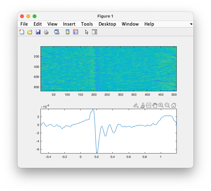
Figure: the ERP image of channel EEG065.
It usually gets more interesting if we sort the trials by reaction time, prestimulus alpha power, or some other metric that influences the ERP responses. Here we can sort them on the trial type.
[triggercode, order] = sort(avg_all.trialinfo(:,1));

figure
subplot(2,1,1); imagesc(squeeze(avg_all.trial(order,367,:)))
subplot(2,1,2); plot(avg_all.time, mean(squeeze(avg_all.trial(:,367,:)),1)); axis tight