workshop / practicalmeeg2025 / handson_mvpa /
Multi-variate pattern analysis (MVPA)
This is a short demonstration on how to do MVPA with FieldTrip. A more elaborate tutorial can be found here.
This tutorial is based on the MVPA-Light toolbox, which is a stand-alone MATLAB toolbox for multivariate pattern analysis involving classification or regression. An alternative toolbox that works well with FieldTrip is ADAM, which has a tutorial paper on the same data as we use here.
The MVPA-Light toolbox features cross-validation, various classifiers, regression models, performance metrics, as well as nested preprocessing and hyperparameter selection. FieldTrip provides a high-level interface to its functions so you do not need to directly interact with the toolbox. However, it needs to be installed and included in MATLAB’s search path. To this end, follow the installation instructions on its GitHub page.
Preparation
We will continue with the dataset that we have been processing during the workshop for subject 15. We read the segmented and preprocessed data from the raw2erp tutorial.
subj = datainfo_subject(15);
filename = fullfile(subj.outputpath, 'raw2erp', subj.name, sprintf('%s_data.mat', subj.name));
load(filename)
We convert the data from a raw representation into a timelocked representation, using the keeptrials option. This results in a 3D array with trials by channels by time.
cfg = [];
cfg.keeptrials = 'yes';
timelock = ft_timelockanalysis(cfg, data);
The trigger codes in timelock.trialinfo can be used to map the trials onto certain conditions or classes.
Famous      = [5 6 7];
Unfamiliar  = [13 14 15];
Scrambled   = [17 18 19];

First_presentation = [5 13 17];
Immediate_repeat   = [6 14 18];
Delayed_repeat     = [7 15 19];

% you can construct your own classes, like faces versus houses, or first versus repeat
classlabel = zeros(size(timelock.trial,1),1);
classlabel(ismember(timelock.trialinfo, Famous))     = 1;
classlabel(ismember(timelock.trialinfo, Unfamiliar)) = 2;
classlabel(ismember(timelock.trialinfo, Scrambled))  = 3;
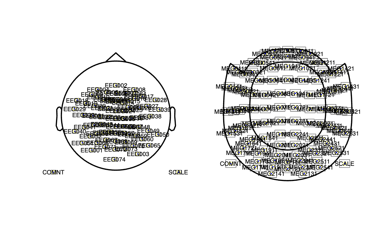
If we want to do the processing on the EEG channels and plot the results, we need the spatial layout for the EEG channels. The spatial layout for the MEG channels is always the same, as the MEG sensors are fixed in the helmet. For the MEG we can therefore use a template layout.
cfg = [];
cfg.elec = timelock.elec;
layout_eeg = ft_prepare_layout(cfg);

cfg = [];
cfg.layout = 'neuromag306mag_helmet.mat';
layout_meg = ft_prepare_layout(cfg);

figure
subplot(1,2,1); ft_plot_layout(layout_eeg) % it could be improved by shifting the electrodes
subplot(1,2,2); ft_plot_layout(layout_meg)
Classifying over channels for each time point
cfg = [];
cfg.method = 'mvpa';
cfg.channel = 'megmag'; % here you can also specify 'meggrad' or 'eeg'
cfg.avgoverchan = 'no';
% cfg.latency = [0.2 0.4];
cfg.avgovertime = 'no';
cfg.design = classlabel;
cfg.features = 'chan';
cfg.mvpa = [];
cfg.mvpa.k = 3;
cfg.mvpa.metric = 'accuracy';
% cfg.mvpa.metric = 'confusion';
% cfg.mvpa.classifier = 'lda'; % for two classes
cfg.mvpa.classifier = 'multiclass_lda';
stat = ft_timelockstatistics(cfg, timelock);
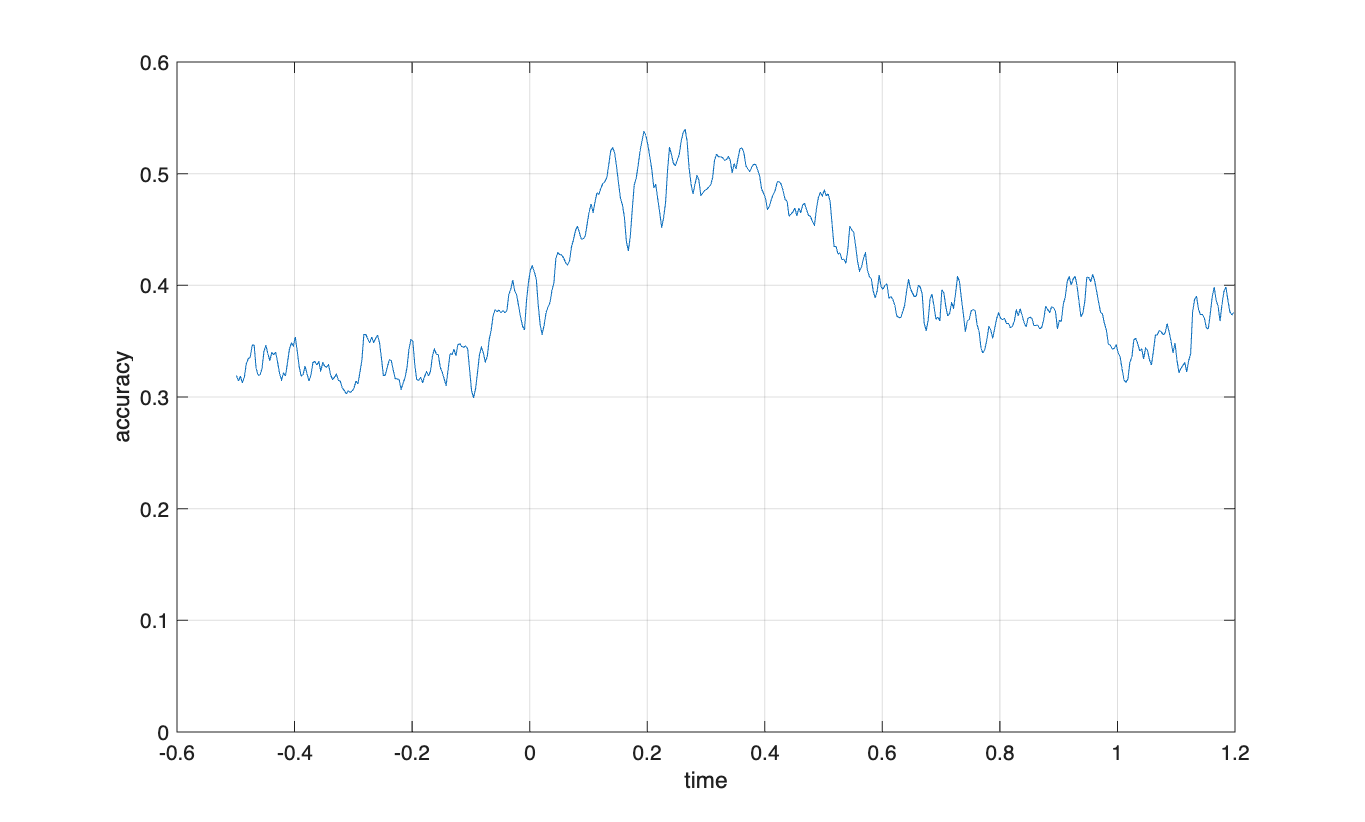
plot(stat.time, stat.accuracy)
xlabel('time')
ylabel('accuracy')
ylim([0 0.6])
grid on
The chance level is 0.33 with a three-class classifier.
Classifying over time for each time channel
cfg = [];
cfg.method = 'mvpa';
cfg.channel = 'megmag'; % here you can also specify 'meggrad' or 'eeg'
cfg.avgoverchan = 'no';
cfg.latency = [0.2 0.4];
cfg.avgovertime = 'no';
cfg.design = classlabel;
cfg.features = 'time';
cfg.mvpa = [];
cfg.mvpa.k = 3;
cfg.mvpa.metric = 'accuracy';
% cfg.mvpa.metric = 'confusion';
% cfg.mvpa.classifier = 'lda';
cfg.mvpa.classifier = 'multiclass_lda';
stat = ft_timelockstatistics(cfg, timelock);
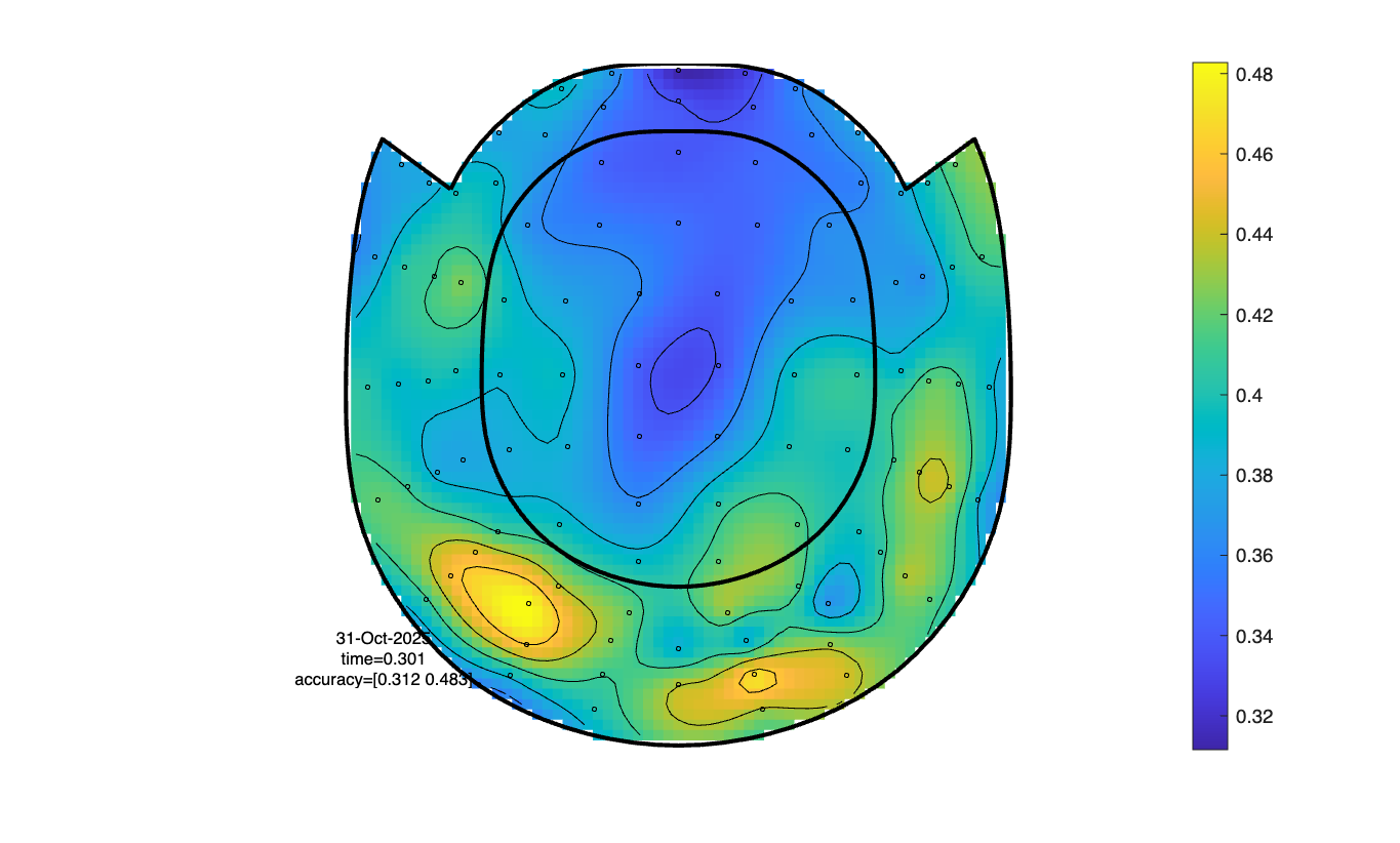
cfg = [];
cfg.parameter = 'accuracy';
cfg.layout = layout_meg; % or layout_eeg, if you use the EEG channels
cfg.colorbar = 'yes';
ft_topoplotER(cfg, stat);
Classifying for each channel and time point
cfg = [];
cfg.method = 'mvpa';
cfg.channel = 'megmag'; % here you can also specify 'meggrad' or 'eeg'
cfg.avgoverchan = 'no';
cfg.latency = 'all';
cfg.avgovertime = 'no';
cfg.design = classlabel;
cfg.features = []; % both time and chan
cfg.mvpa = [];
cfg.mvpa.k = 3;
cfg.mvpa.metric = 'accuracy';
% cfg.mvpa.metric = 'confusion';
% cfg.mvpa.classifier = 'lda';
cfg.mvpa.classifier = 'multiclass_lda';
stat = ft_timelockstatistics(cfg, timelock);
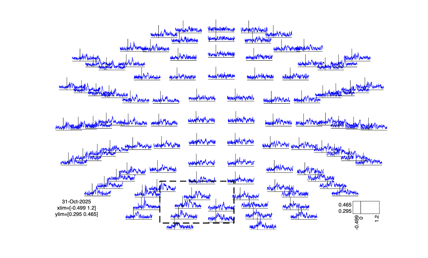
cfg = [];
cfg.parameter = 'accuracy';
cfg.layout = layout_meg; % or layout_eeg, if you use the EEG channels
cfg.colorbar = 'yes';
ft_multiplotER(cfg, stat);
The figure is interactive and you can make a selection in the figure and zoom in on certain channels and/or time windows.
Suggested further reading
You can find more details on multi-variate pattern analysis in this tutorial.