Coregistration of Optically Pumped Magnetometer (OPM) data

Introduction

Conventionally, MEG is recorded with SQUIDs, which are superconductive sensors that require cryocooling and hence need to be placed as an fixed helmet-shaped array in a dewar. Optically Pumped Magnetometers (OPMs) are a new type of magnetic field sensors for MEG. OPMs do not require cryocooling and can be placed individually. Due to their small size and flexibility, different strategies are used to place OPM sensors on the head.

For a good interpretation of the MEG signals recorded with the OPM sensors over the head, it is important to coregister the OPM sensors (location and orientation) with the head. Also for source reconstruction it is required to coregister the sensors with the anatomical MRI, the volume conduction model, and the source model. Whereas SQUID-based MEG systems come with standard and coregistration procedures, for OPMs there is not a single standard.

Some labs use flexible caps to place the OPMs, similar to EEG and fNIRS caps. These flexible caps don’t constrain the orientation of the sensors very well, which means that the sensor orientation relative to the head can change during the experiment depending on the head orientation and that the sensors can wobble due to movement. Since the magnetic field measured with MEG is a vector, the measurement is sensitive to these orientation differences.

To ensure a well-defined sensor placement, labs also often use helmets to position the OPM sensors relative to the head. These helmets can be designed and 3-D printed to fit optimally to the individual head, or can be designed as standard helmets to fit multiple participants (with different sized helmets for children and adults).

This tutorial demonstrates different methods for coregistering OPM sensors. Each method is demonstrated including data that you can download to carry out all steps yourself. Furthermore, it discusses the advantages and disadvantages of each method.

In this tutorial we will not consider the coregistration of OPM sensors in flexible EEG-like caps. This tutorial will also not cover the processing of the MEG signals recorded from the participants brain, that is covered in the tutorial on preprocessing of OPM data.

Background

The common aim of the coregistration methods that we explore in this tutorial is to align geometrical objects - ‘things’ that have a position and orientation in 3D space - with respect to one another. Ultimately, we want know the location of the OPM sensors relative to the participant’s head and brain.

In the examples below, the OPM sensor positions and orientations are initially expressed in a coordinate system relative to the FieldLine smart helmet. To facilitate the downstream analysis of the MEG signals, e.g., for group level analysis, it is customary to aim for the OPM sensors expressed in a coordinate system that is defined based on anatomical landmarks on the participant’s head.

The dataset used in this tutorial

The data for this tutorial was recorded with a 32-sensor FieldLine HEDscan v3 system with a so-called smart helmet. It can be downloaded from our download server.

Procedure

This tutorial describes different ways to achieve coregistration:

• Using geometric information from a Polhemus 3D tracker, matching two sets of points that are known to match one-to-one.
• Using head localization coils, where the location of the coils on the head is known, and the location of the coils relative to the sensors can be calculated.
• Using an optical 3D scan of the head and helmet, and aligning this with an anatomical MRI and template sensor positions.
• Using sensor-depth information from the FieldLine smart helmet as a proxy for the head surface.
• Using individually designed 3D printed helmets

Procedural outlines of each of the examples are provided in more detail below.

Coregistration using a Polhemus tracker

The following example is based on a Polhemus recording, which - besides a measurement of some points on the participant’s head surface - contains the digitized locations of 8 small indentations that serve as landmarks on the FieldLine smart helmet. These 8 fixed locations are also defined in the fieldlinebeta2 template helmet, but there expressed in a different coordinate system.

The procedure for this consists of the following steps:

• Read in the headshape and change the coordinate system, using ft_read_headshape and ft_convert_coordsys. For visualization we use ft_plot_headshape and ft_plot_axes.
• Identification of the reference points in the Polhemus measurement
• Reading the template sensor positions using ft_read_sens
• Calculation of the transformation parameters, using ft_electroderealign.
• Apply the transformation to the template sensors, using ft_transform_geometry, and ft_plot_sens for visualization.

Read the Polhemus file and impose a head-based coordinate system

This specific Polhemus measurement has been obtained as a pilot at the DCCN with the reference sensor mounted on plastic safety glasses. Since the safety glasses were too bulky to fit under the MEG helmet, we secured them around the neck of the participant. A more appropriate procedure could have been implemented by using smaller safety glasses that would fit under the OPM helmet, or by separating the reference sensor from the glasses and taping it straight onto the forehead of the participant.

The Polhemus recording was done using the CTF software. The software requires the experimenter to click the left ear, the right ear, and the nasion. It then expresses all subsequent points according to the CTF convention for the definition of the X/Y/Z axes of the coordinate system, which is anterior-left-superior (ALS).

For consistency with the other examples in this tutorial, we will first convert the head-based coordinate system to be right-anterior-superior (RAS).

%% read in the data and enforce the units to be in 'mm'
headshape = ft_read_headshape('example1_head_markers.pos');
headshape = ft_convert_units(headshape, 'mm');

%% visualization, coordinate axes are initially ALS
figure
ft_plot_headshape(headshape)
ft_plot_axes(headshape)
view([-27 20])

If you 3D rotate the figure, you can recognize the nose; it is just below the red +X (unknown) axis.

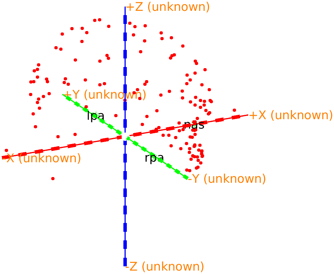
Figure: Polhemus recorded headshape with the coordinate axes according to the CTF-convention: the X-axis is pointing towards the nose.

From the figure we can see that the first X axis pointing to the nose or anterior, the second Y axis is pointing to the left, and the third Z axis is pointing to superior. Hence we refer to this as an ALS coordinate system. In fact, closer inspection reveals that the origin is exactly between the two ears, which means that it is consistent with the CTF coordinate system. This is information we can add to the data structure to facilitate automatic coordinate system conversion.

headshape.coordsys = 'ctf';
headshape = ft_convert_coordsys(headshape, 'neuromag');  % this rotates it such that the X-axis points to the right

%% visualization, coordinate axes are now RAS
figure
ft_plot_headshape(headshape)
ft_plot_axes(headshape)
view([114 20])

The nose is now just below the green +X axis, which now also specifies that it corresponds to the anterior direction. The ft_plot_axes function automatically adds these labels whenever an object specifies the coordinate system. You can click in the figure with the right mouse button and change the view to any of top/bottom, left/right, and front/back.

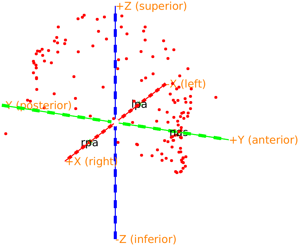
Figure: Adjusted headshape expressed in the RAS coordinate system.

Identification of reference points

The Polhemus file not only describes the shape of the head and face, but also a number of reference points on the helmet. You can recognize them in the previous figure that you made, especially if you rotate it such that you see the head from the top. There are 8 points visible that have a clear distance from the head surface.

The reference points correspond to the last 8 points that were digitized. The order in which they were digitized was written down on a piece of paper: first left, from front-to-back, then right, from front-to-back. The points on the FieldLine helmet are indicated as A1-A8, and the order in which they were recorded is therefore ‘A5’, ‘A6’, ‘A7’, ‘A8’, ‘A1’, ‘A2’, ‘A3’, ‘A4’. As we know where the points are in the Polhemus recording and in the helmet definition, we can calculate the transformation parameters to move these points from the helmet coordinate system to the coordinate system that is defined within the Polhemus measurement. The same transformation can then be applied to the OPM sensors.

%% select the reference points on the helmets, with their corresponding label
fid_measured = [];
fid_measured.pos(1,:) = headshape.pos(end-7,:);
fid_measured.pos(2,:) = headshape.pos(end-6,:);
fid_measured.pos(3,:) = headshape.pos(end-5,:);
fid_measured.pos(4,:) = headshape.pos(end-4,:);
fid_measured.pos(5,:) = headshape.pos(end-3,:);
fid_measured.pos(6,:) = headshape.pos(end-2,:);
fid_measured.pos(7,:) = headshape.pos(end-1,:);
fid_measured.pos(8,:) = headshape.pos(end-0,:);
fid_measured.label = {'A5', 'A6', 'A7', 'A8', 'A1', 'A2', 'A3', 'A4'};

To perform a later comparison, it is convenient to sort them from 1 to 8.

[fid_measured.label, indx] = sort(fid_measured.label);
fid_measured.pos = fid_measured.pos(indx,:);

We can explicitly add the fiducials to the data structure that describes the head shape. The ft_plot_headshape function will in that case explicitly plot them, including their labels.

headshape.fid = fid_measured

We also have the template specification of the OPM sensor locations with the corresponding set of reference points for the FieldLine beta 2 helmet. The ft_plot_sens function will also plot the reference points or fiducials.

fieldlinebeta2 = ft_read_sens('fieldlinebeta2.mat'); % from fieldtrip/template/grad
fieldlinebeta2 = ft_convert_units(fieldlinebeta2, 'mm');
fid_helmet     = fieldlinebeta2.fid;

%% show the misalignment
figure
ft_plot_headshape(headshape)
ft_plot_axes(headshape)
ft_plot_sens(fieldlinebeta2)
view([102 5]);

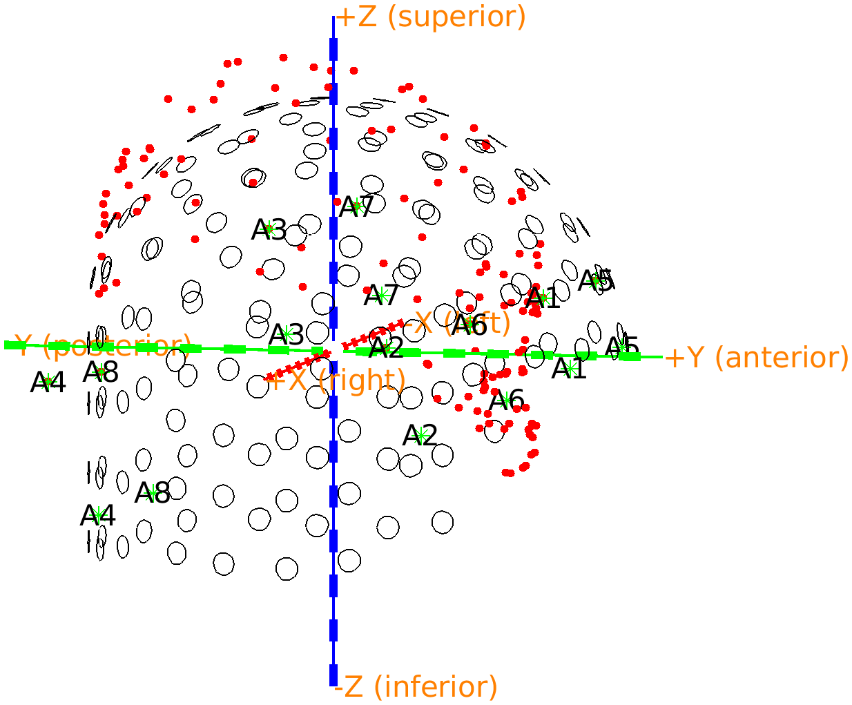
Figure: The reference points of the Polhemus measurement are not aligned with those of the OPM helmet; you can see the head stick out at the top of the helmet.

We will proceed with ft_electroderealign, which was originally implemented to align EEG electrode positions to a head surface. As it turns out, it can also be used more general to align two sets of points.

Calculation of the transformation parameters

The alignment parameters can be estimated using the template method in ft_electroderealign. Since we want to express the OPM sensors’ coordinates in the head coordinate system, the Polhemus measured positions will be used as the target.

%% estimate the alignment parameters
cfg         = [];
cfg.method  = 'template';
cfg.target  = fid_measured;
cfg.elec    = fid_helmet;
fid_aligned = ft_electroderealign(cfg);

Apply the transformation to the OPM sensors

The output data structure fid_aligned not only contains the aligned fiducials, but also the parameters that were used to align (or transform) them. We can apply the same transformation parameters to the OPM sensors.

fieldlinebeta2_head = ft_transform_geometry(fid_aligned.rigidbody, fieldlinebeta2, 'rigidbody');

figure
ft_plot_headshape(headshape)
ft_plot_axes(headshape)
ft_plot_sens(fieldlinebeta2_head)
view([102 5]);

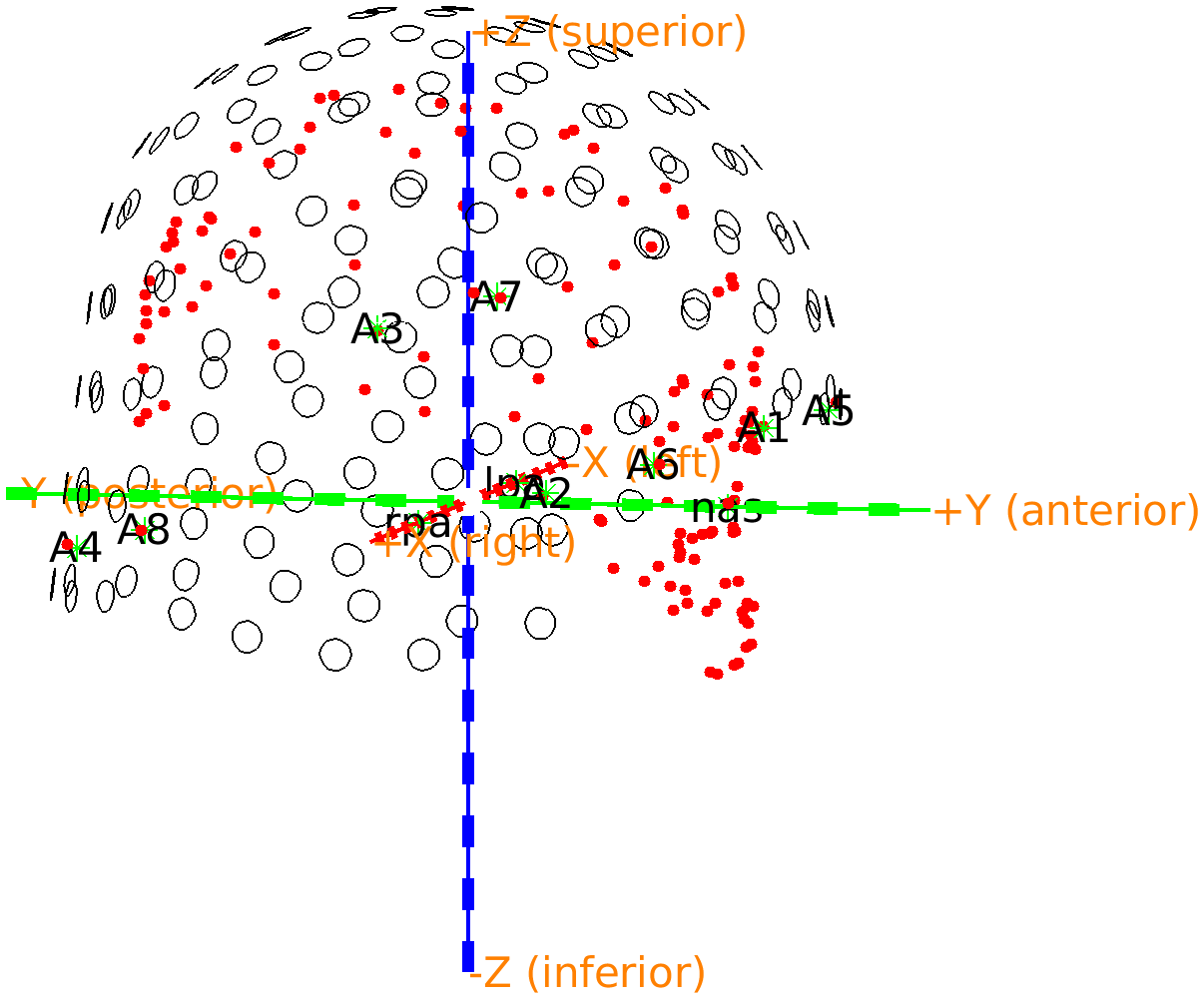
Figure: OPM sensor locations are in register with the Polhemus headshape.

If you rotate the image, the first thing to notice is that the nose is properly pointing towards the opening of the helmet where the face should be. Furthermore, careful inspection shows that there are now two sets of overlapping fiducials. Since we made sure previously that the fiducials are sorted from 1 to 8, we can compute the difference between the positions in the aligned helmet and the Polhemus measurement. The reason for the overlap not being perfect is that the Polhemus measurement has some inaccuracies, both in placing the stylus, and in the digitization process.

fieldlinebeta2_head.fid.pos - headshape.fid.pos
ans =
    0.3611    0.2083   -0.0140
    4.8747    1.9590    1.6937
    1.9225    0.0960    1.0279
   -1.0412    2.4382   -0.8980
    0.6837   -2.4648   -2.2817
   -2.8585   -2.4431   -0.3389
   -2.0272   -1.7663    0.5568
   -1.9592    0.4899    0.2620

Coregistration using head localizer coils

Conventional SQUID-based MEG systems are based on certain number of sensors (e.g., 275 or 306) placed in a fixed-size helmet to accommodate most participants. Unless when using custom headcasts, the SQUID MEG helmet gives the participant a few cm of space around the head. The heads of different participants will therefore not be in the same position relative to the helmet, for an individual participant the position of the head in the helmet will differ between sessions, and can even vary within a session. Conventional SQUID-based MEG systems therefore commonly use head localization coils (HLC) or head position indicator (HPI) coils.

The HPI coils are placed on the head - usually on well-defined anatomical landmarks - and at the start of the recording session a small current is passed through the coils to create small magnetic dipoles. Sometimes the localization is repeated at the end of the recording session, and some systems also have the possibility to do the localization continuously. These magnetic dipoles can be localized, thereby determining the position of the sensors relative to the anatomical landmarks. All commercial SQUID-based MEG systems have a standard procedure for this that is well-integrated in the acquisition protocol and software, consequently the MEG recordings stored by the acquisition software include the sensor positions in head coordinates.

OPM sensors allow for individual placement and use variable-sized helmets. Furthermore, labs that operate an OPM MEG system will not all have the same number of sensors; some labs have as few as 8 sensors, whereas other labs might have up to 128 sensors.

The dataset used here contains 32 channels, with the OPM sensors relatively uniformly distributed over the 144 slots of the FieldLine beta 2 helmet. We did not perform the measurement on a real participant’s head, but rather used the CTF magnetic phantom, which is basically a plexiglass mount to which the HPI coils can be attached at fixed and known locations. To maximize the coverage of the coils, the phantom head was positioned quite high into the helmet.

We will analyze a ~1 minute segment of data during which the 3 HPI coils were energized with 3 sine wave signals at different frequencies: at 8 Hz for the ‘nasion’ coil, 11 Hz for the ‘right ear’ coil, and 14 Hz for the ‘left ear’ coil. These sine waves are orthogonal, i.e., uncorrelated in time. When the data is bandpass filtered, we can get the signal generated by each of the individual coils. Subsequently we can fit dipoles to the spatial topography of the first principal component of the bandpass-filtered data.

The procedure for this consists of the following steps:

• To evaluate the MEG signal and the spectrum, we start off with ft_preprocessing, ft_databrowser, ft_selectdata and ft_freqanalysis.
• Processing of the data to get the contribution of each individual HPI coil, using ft_preprocessing, .
• Fitting of dipoles to the topographies of the first principal components of the bandpass filtered data, using ft_componentanalysis, and ft_dipolefitting. For visualization of the spatial topographies, we use ft_topoplotIC, and for the dipole fit we start with a grid search, and we use ft_prepare_sourcemodel to create the search grid.
• Calculation of the transformation matrix that moves the sensors to the head-based coordinate system, using ft_headcoordinates.
• Apply the transformation matrix to the sensors, using ft_transform_geometry.

Processing of the data to capture the signal of the HPI coils

% load in the data
cfg              = [];
cfg.dataset      = 'example2_magneticphantom_HPIplusdipoleset6_raw.fif';
cfg.coilaccuracy = 0;
data_all         = ft_preprocessing(cfg);

We can visualize the data with ft_databrowser to see where the sine-wave signals start and end.

cfg = [];
cfg.viewmode = 'vertical';
cfg.blocksize = 300; % seconds
ft_databrowser(cfg, data_all);

You can recognize four blocks of about 60 seconds each, followed by a final block of about 60 seconds in which you don’t see much. In the first block all three coils were energized at the same time, at different (orthogonal) frequencies. That is the part of the data that we will use. A bit later in the recording each of the coils was energized individually; those pieces of data would have been useful if all coils would have been driven with the same frequency. In the last block the magnetic dipole that is at the center of the CTF phantom was energized at 11 Hz; the signal there is much weaker since the coil is further away from the OPM sensors.

We cut out the relevant time segment using ft_selectdata. After this step the data is exactly 300000 samples long (60 seconds times 5000 samples/second).

% this is the time of a single sample
tsample = 1./data_all.fsample

cfg         = [];
cfg.latency = [0 60-tsample];
cfg.channel = {'all' '-L212_bz' '-R212_bz'};
data        = ft_selectdata(cfg, data_all);

We cut the data into 10-second segments with 80% overlap and compute the averaged powerspectrum over all segments to verify the expected spectral peaks (and their harmonics) at 8, 11 and 14 Hz.

cfg            = [];
cfg.length     = 10;
cfg.overlap    = 0.8;
data_segmented = ft_redefinetrial(cfg, data);

cfg           = [];
cfg.method    = 'mtmfft';
cfg.foilim    = [0 40];
cfg.taper     = 'dpss';
cfg.tapsmofrq = 0.2;
cfg.pad       = 10;
freq          = ft_freqanalysis(cfg, data_segmented);

figure;
plot(freq.freq, log10(mean(freq.powspctrm)));
xlabel('frequency (Hz)');
ylabel('log_10 power')

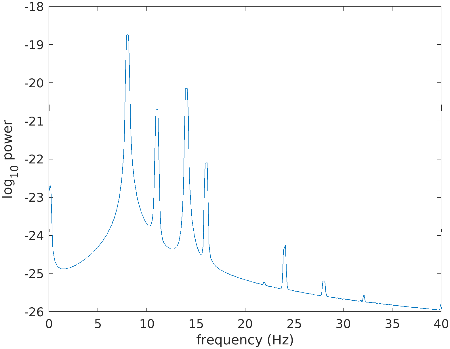
Figure: Powerspectrum from a measurement containing strong signals at 8, 11 and 14 Hz, and at their harmonics.

To focus on the signals of the specific HPI-coils, we bandpass filter the data in the frequency bands corresponding to each of the coils, and cut off the edges for any potential filter edge artifacts.

cfg            = [];
cfg.bpfilter   = 'yes';
cfg.bpfilttype = 'firws';
cfg.usefftfilt = 'yes';
cfg.bpfreq     = [7 9];
data08         = ft_preprocessing(cfg, data); % nas

cfg.bpfreq     = [10 12];
data11         = ft_preprocessing(cfg, data); % rpa

cfg.bpfreq     = [13 15];
data14         = ft_preprocessing(cfg, data); % lpa

cfg            = [];
cfg.latency    = [4 56-1./data.fsample];
data08         = ft_selectdata(cfg, data08);
data11         = ft_selectdata(cfg, data11);
data14         = ft_selectdata(cfg, data14);

%% look at 2 seconds of the data
figure;
plot(data08.time{1}, data08.trial{1});
xlim([4 6]);
xlabel('time (s)');
ylabel('magnetic field strength (T)');

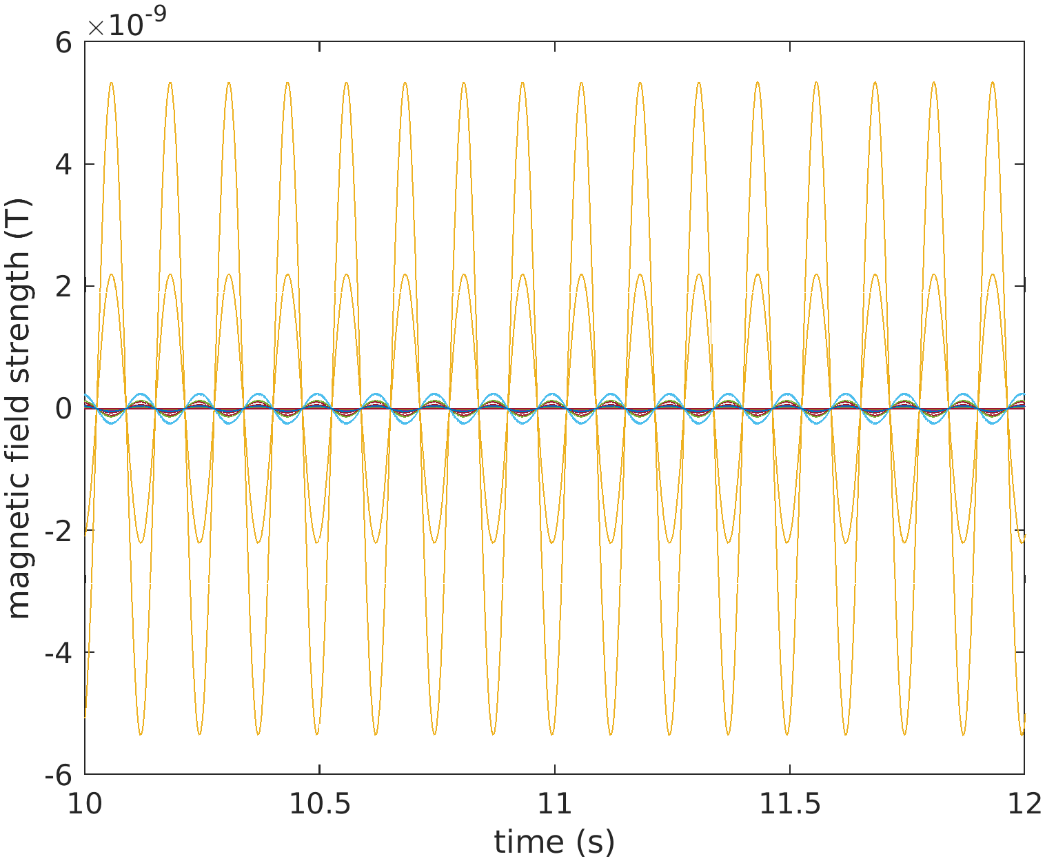
Figure: Two seconds of data, bandpass filtered around 8 Hz.

Fit dipoles to the sensor topographies

We proceed by performing a principal component analysis (PCA) on the filtered data. The idea is that - given that the signals from the HPI coils are the strongest signals in the measurement, and given that we have bandpass filtered the data - the strongest principal components will represent the ‘spatial fingerprints’ of each of the HPI coils. Those fingerprints will be used to perform a dipole fit, i.e., find the position of a dipole that optimally explain those principal components.

cfg            = [];
cfg.method     = 'pca';
cfg.updatesens = 'no';
comp08 = ft_componentanalysis(cfg, data08);
comp11 = ft_componentanalysis(cfg, data11);
comp14 = ft_componentanalysis(cfg, data14);

%% look at the topographies
cfg              = [];
cfg.component    = 1;
cfg.layout       = 'fieldlinebeta2bz_helmet.mat';
cfg.gridscale    = 150;
cfg.interplimits = 'sensors';
cfg.figure       = subplot('position',[0 0 1/3 1]);
ft_topoplotIC(cfg, comp08);
cfg.figure       = subplot('position',[1/3 0 1/3 1]);
ft_topoplotIC(cfg, comp11);
cfg.figure       = subplot('position',[2/3 0 1/3 1]);
ft_topoplotIC(cfg, comp14);

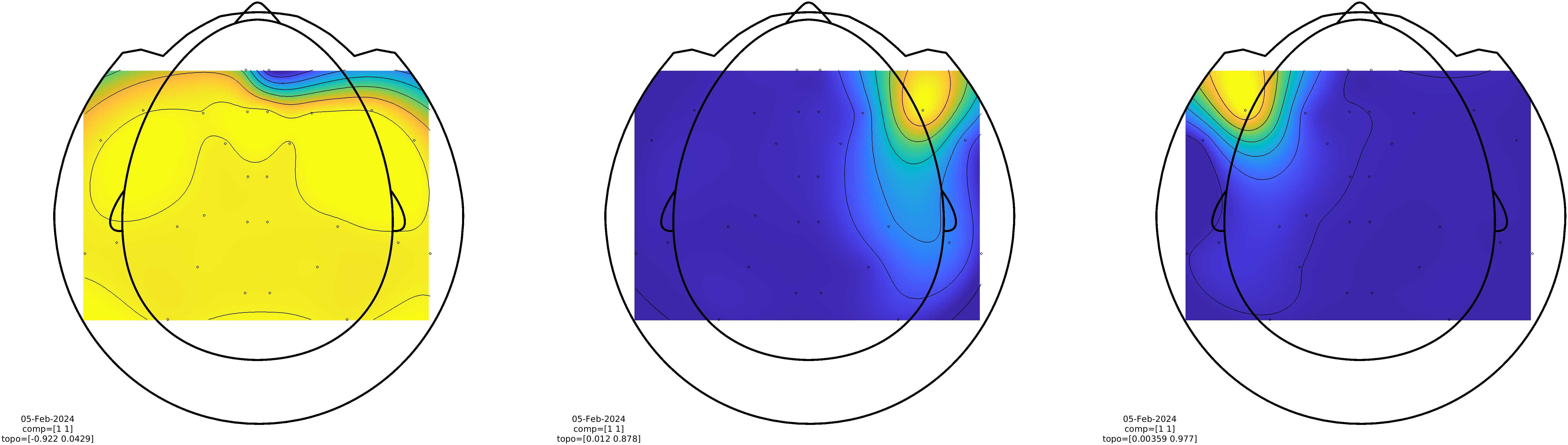
Figure: Spatial topographies of the signals generated by the 3 HPI coils.

For the fitting the magnetic dipole positions, we will use a grid search as an initial scan over the whole volume, followed by a iterative non-linear optimization. The grid search is motivated by the fact that a non-linear search of the whole parameter space (i.e., volume of space covered by the helmet) might result in convergence to a local minimum.

The following creates a sourcemodel that consists of a regular grid of dipole positions that will be used for the initial grid search.

%% create a regular grid of dipole positions bounded by the helmet
fieldlinebeta2 = ft_read_sens('fieldlinebeta2.mat');  % from fieldtrip/template/grad

% make a fake headshape, we use this to make a fake headmodel
fake_headshape      = [];
fake_headshape.pos  = fieldlinebeta2.coilpos;
fake_headshape.unit = 'm';

% create a fake singleshell headmodel, this will act as the boundary for the grid
cfg = [];
cfg.method = 'singleshell';
cfg.headshape = fake_headshape;
cfg.numvertices = 144; % keep the same number of vertices as OPMs
fake_headmodel = ft_prepare_headmodel(cfg);

%% create the grid, grid points outside the fake head will be flagged as such
cfg            = [];
cfg.headmodel  = fake_headmodel;
cfg.resolution = 0.0075;
sourcemodel    = ft_prepare_sourcemodel(cfg);

% this is the real volume conductor model that we want to use
cfg = [];
cfg.method = 'infinite';
headmodel = ft_prepare_headmodel(cfg);

Now we can perform the dipole fits.

cfg             = [];
cfg.headmodel   = headmodel;
cfg.grad        = data.grad;
cfg.component   = 1;
cfg.gridsearch  = 'yes';
cfg.sourcemodel = sourcemodel;
dip08 = ft_dipolefitting(cfg, comp08);
dip11 = ft_dipolefitting(cfg, comp11);
dip14 = ft_dipolefitting(cfg, comp14);

The data in this example was obtained with the HPI coils placed on well-defined locations on the CTF magnetic phantom. The phantom, when seen from above, has the Nasion coil located at 12:00 o’clock and LPA and RPA at 9:00 and 3:00 o’clock. The radius of the phantom is 7.5 cm. Also accounting for the thickness of the coils, the expected distances between the localizer coils on the phantom are as follows:

• LPA-RPA should be 15.32 cm
• Nasion-LPA and Nasion-RPA should be 10.83 cm

We can verify the reconstructed distances as follows. Note that for a real measurement, one would need to measure the distance between the fiducials first (e.g., with a Polhemus scanner, see above) in order to be able to make such a comparison.

% for verification
disp(norm(dip11.dip.pos - dip14.dip.pos)*100) % in cm
disp(norm(dip08.dip.pos - dip11.dip.pos)*100)
disp(norm(dip08.dip.pos - dip14.dip.pos)*100)

15.4760
10.2201
10.5455

Definition of the head-based coordinate system

Now that we have identified the HPI coil locations, we can compute the coregistration matrix that transforms the HPI coil positions from ‘helmet’ coordinates to ‘head’ coordinates. Here, we use the neuromag convention.

% transform fiducial coordinates to head coordinates (RAS)
fid1 = dip08.dip.pos; % nas
fid2 = dip14.dip.pos; % lpa
fid3 = dip11.dip.pos; % rpa
transform_sens2head = ft_headcoordinates(fid1, fid2, fid3, 'neuromag');

Apply the transformation matrix to the sensors

Converting the actual OPM positions from ‘helmet’ or sensor coordinates to ‘head’ coordinates is done using the ft_transform_geometry function.

fieldlinebeta2_head = ft_transform_geometry(transform_sens2head, fieldlinebeta2);

We can plot the sensors, which are now in head coordinates

figure
ft_plot_sens(fieldlinebeta2_head)
ft_plot_axes(fieldlinebeta2_head)
view([130 30]);

and if we transform the dipole positions from helmet to head coordinates, we can also add those to the figure.

ft_plot_dipole(dip08.dip.pos, dip08.dip.mom, 'length', 0.02, 'diameter', 0.01)
ft_plot_dipole(dip11.dip.pos, dip11.dip.mom, 'length', 0.02, 'diameter', 0.01)
ft_plot_dipole(dip14.dip.pos, dip14.dip.mom, 'length', 0.02, 'diameter', 0.01)

Note that the HPI coils were placed on the CTF magnetic dipole phantom, which was rather placed deep into the helmet. As such the HPI coils or dipoles at NAS, LPA and RPA are not really on positions where the real nose and ears would be.

Coregistration using a 3D scanner

The procedure that we follow here is published in Zetter et al. 2019. An optical 3D scanner can be used to capture the participant’s facial features combined with the OPM helmet. The face from the 3D scan can be coregistered with a 3D model of the face obtained from the individual’s anatomical MRI. Similarly, the helmet from the 3D can be coregistered with a 3D model of the helmet. Thus, the optical 3D scan serves as an intermediary to link the face and anatomical MRI to the helmet and sensors.

The procedure for this consists of the following steps:

• Read the 3D scan, assign a meaningful coordinate system, and erase the irrelevant parts, using ft_read_headshape, ft_meshrealign, and ft_defacemesh.
• Read the anatomical MRI, assign a well defined head coordinate system, using ft_read_mri, and ft_volumerealign.
• Interactive alignment of the face - extracted from the 3D scan - with the face extracted from the anatomical MRI, using ft_volumesegment, ft_prepare_mesh, and ft_meshrealign.
• Interactive alignment of the helmet - extracted from the 3D scan - with the reference helmet and sensors, using ft_meshrealign.
• Combination of the obtained alignment parameters into a single transformation matrix
• Application of the resulting transformation to the sensor array, using ft_transform_geometry.

Processing the optical 3D scan

We read in the model from the optical 3D scanner. The first step is to coregister the 3D scan with a coordinate system that has its axes pointing into more or less canonical directions (relative to the participant). In the next step we remove irrelevant parts of the image, such as the back of a chair. Then we separate the ‘face’ part from the ‘helmet’ part to facilitate their respective alignments.

scan      = ft_read_headshape('example3_face_helmet.obj');
scan.unit = 'm'; % the estimated 'dm' is not correct

figure; hold on;
ft_plot_headshape(scan);
ft_plot_axes(scan);
lighting gouraud
material dull
light

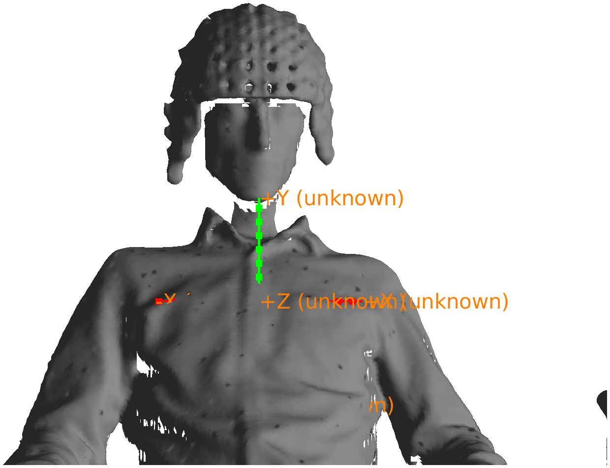
Figure: 3D scan with a not so clearly defined coordinate system.

In the example scan, the coordinate axes’ orientations relative to the participant are not cleary defined. The origin [0, 0, 0] is somewhere in the chest, but the axes are reasonably well-behaved, i.e., pointing approximately along the left/right, anterior/posterior, and superior inferior directions. However, this will depend on the 3D scanner and the angle from which you start the scan.

To facilitate later processing, we will assign a better defined coordinate system to the scan, focussing on the head. The exact coordinate system does not really matter, but it is convenient to use a coordinate system such that the X/Y/Z axes are pointing approximately in the same direction as the head coordinate system that we will use for the MRI the subsequent analyses. The coordinate system that we aim for in the subsequent analysis is RAS (Right, Anterior, Superior) and hence we specify cfg.coordsys='neuromag' which allows us to approximately indicate the N(asion), the L(eft) preauricular point, and the R(ight) preauricular point. Since the participant’s ears are not visible in the scan, we will use the protruding points on the helmet’s rim to define ‘L’ and ‘R’.

% approximately align the mesh to a RAS coordinate system,
% by clicking on 'dummy' nas/lpa/rpa
cfg          = [];
cfg.method   = 'fiducial';
cfg.coordsys = 'neuromag';
scan         = ft_meshrealign(cfg, scan);

figure; hold on;
ft_plot_headshape(scan);
ft_plot_axes(scan);
view([125 10]);
lighting gouraud
material dull
light

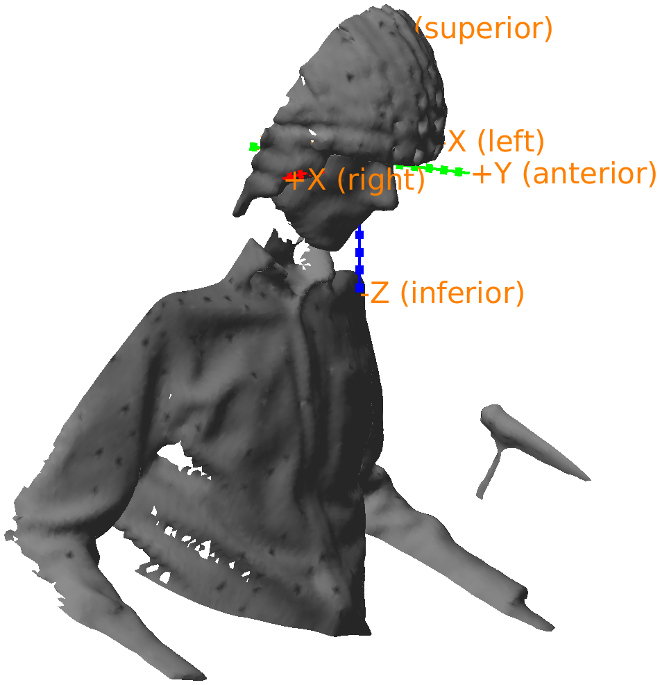
Figure: 3D scan with a coordinate system relating to the head and helmet.

load example3_face_helmet_aligned.mat  % this contains the aligned scan

In the example scan, a large part of the body of the participant is also present. We remove it to facilitate the alignment. The below code uses ft_defacemesh with cfg.method='plane'. This particular method discards parts of the scan that are on one side of the plane, which is indicated by the direction of the stick that is sticking out from the middle of the plane. By setting the viewpoint in the interactive window to ‘right’, we get a convenient view to specify the plane. Note that the viewpoint does not have a consequence for the points to be excluded. Here, good results were obtained by using the following numbers to define the cutting plane: rotate [-40 0 0], translate [0 0 -140].

% cut off the irrelevant parts
cfg         = [];
cfg.method  = 'plane';
scan_head   = ft_defacemesh(cfg, scan); % viewpoint left,  rotate [-30 0 0], translate [0 0 -130];

figure; hold on;
ft_plot_headshape(scan_head);
ft_plot_axes(scan_head);
view([125 10]);
lighting gouraud
material dull
light

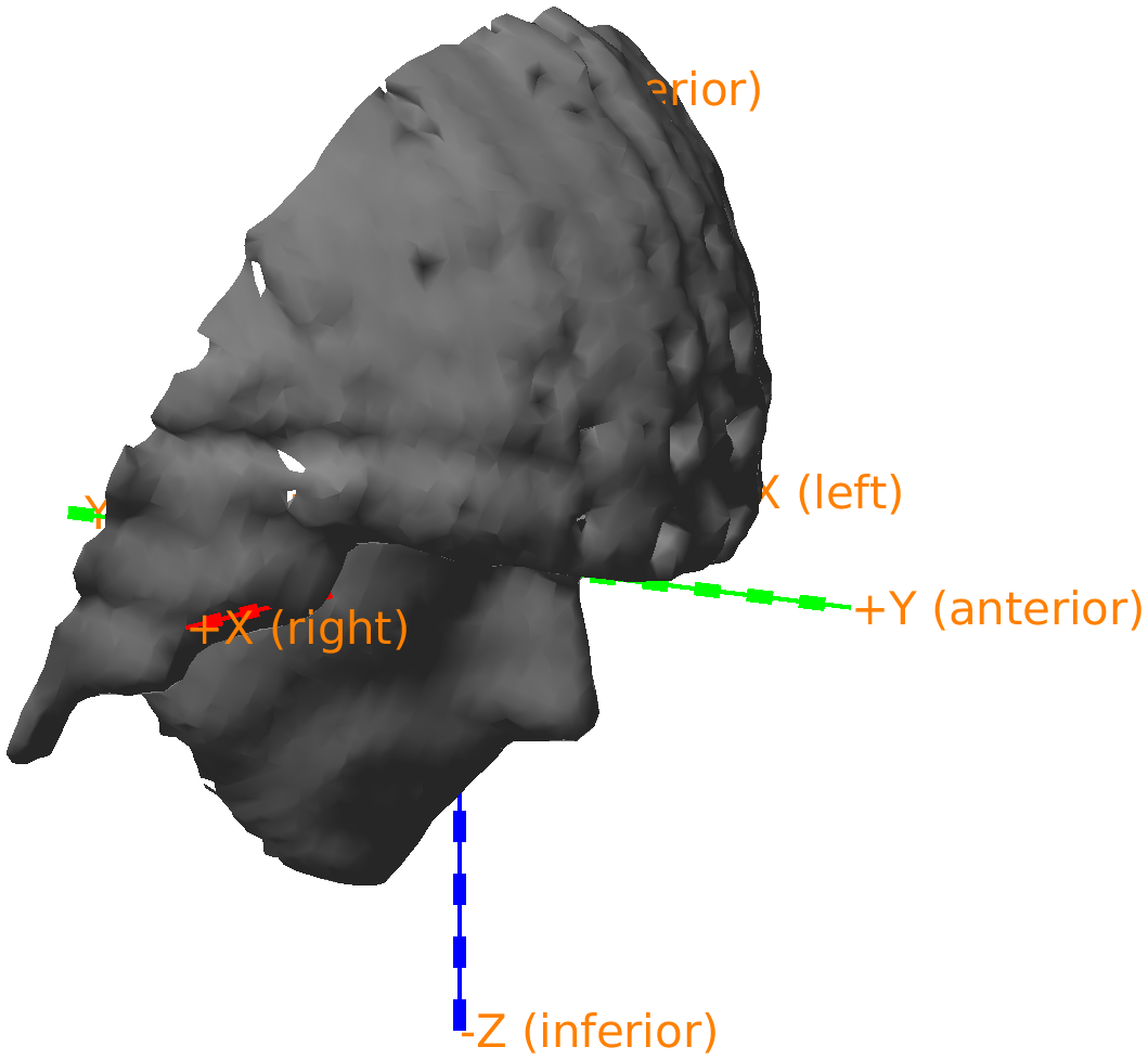
Figure: 3D scan with only the face and helmet.

In the following, we separate the ‘helmet’ part of the scan from the ‘face’ part, because this facilitates the alignment performed below. Note that we need to ensure that any change in the coordinates of one of these objects should be reflected in the other object as well. Clearly, this is needed because the 3D scan of the two objects is the crucial link from facial anatomy towards sensors.

% separate the face from the helmet, it's easier to keep the face at first
% instance, and then go back to the original mesh to get the helmet

cfg        = [];
cfg.method = 'box';
cfg.selection = 'inside';
scan_face  = ft_defacemesh(cfg, scan_head); % rotate [-30 0 0], scale [0.15 0.20 0.20], translate [3 0 -80]

figure; hold on;
ft_plot_headshape(scan_face);
ft_plot_axes(scan_face);
view([125 10]);
lighting gouraud
material dull
light

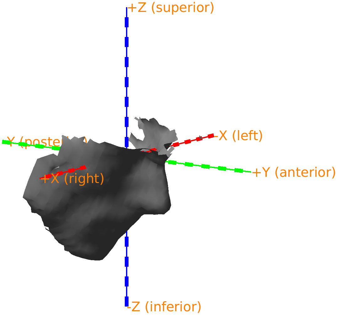
Figure: 3D scan with only the face.

The surface mesh of the helmet will be extracted by removing the face from the scan. We use the same selection as in the extraction of the face, but now we keep the outside of the box rather than the inside.

cfg           = [];
cfg.method    = 'box';
cfg.selection = 'outside';
scan_helmet   = ft_defacemesh(cfg, scan_head); % rotate [-30 0 0], scale [0.15 0.20 0.20], translate [3 0 -80]

figure; hold on;
ft_plot_headshape(scan_helmet);
ft_plot_axes(scan_helmet);
view([125 10]);
lighting gouraud
material dull
light

Figure: 3D scan with only the helmet.

Processing of the anatomical MRI

Here, we read in the anatomical MRI and define the coordinate system based on the conventions typical for SQUID-based MEG. Using anatomical landmarks on the surface of the head, a coordinate system is defined. The same coordinate system can also be defined using a Polhemus tracker (as in coregistration strategy 1, see above). Alternatively, an ACPC coordinate system could have been defined based on anatomical structures in the brain (cf. the anterior and posterior commissures), which facilitates spatial alignment and normalization across participants and comparison with fMRI data.

After reading in the MRI, you can check the coordinate system with ft_determine_coordsys.

% read in the anatomical MRI
mri = ft_read_mri('example3_anatomical.nii');

% check the coordinate system
ft_determine_coordsys(mri, 'interactive', 'no');

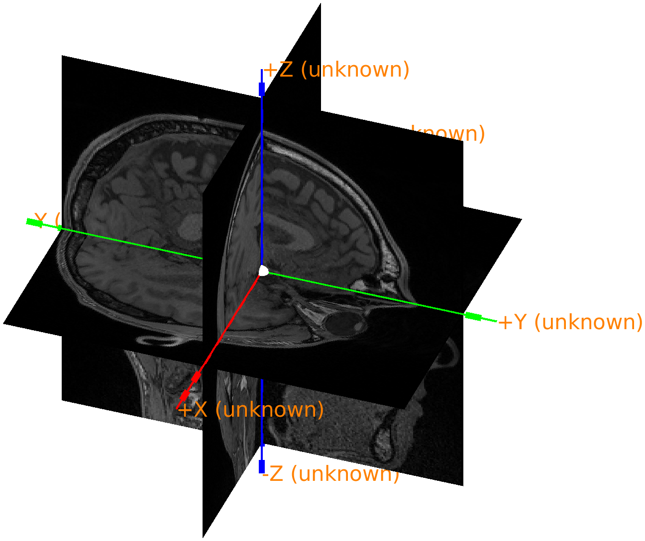
Figure: anatomical MRI in the original scanner coordinates.

As the above figure shows, the axes are labeled as ‘unknown’, but it seems that they are oriented according to the RAS convention, while the origin of the coordinate system is ill-defined, as that depends how the subject was lying in the MRI scanner and how the scanned volume was configured.

We will explicitly align the MRI to an anatomical landmark-based coordinate system next, which requires interactive identification of the relevant landmarks (Nasion, Left, and Right pre-auricular points).

% define a head coordinate system linked to the anatomical landmarks
cfg           = [];
cfg.coordsys  = 'neuromag';
mri_realigned = ft_volumerealign(cfg, mri);

% check the coordinate system after realignment
ft_determine_coordsys(mri_realigned, 'interactive', 'no');

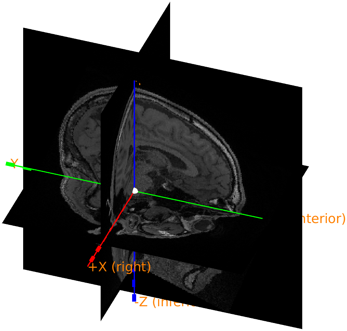
Figure: anatomical MRI image with a ‘neuromag’ head coordinate system.

load example3_mri_realigned.mat % this contains the realigned mri

Alignment of the 3D scan face with the MRI

We can extract the scalp surface from the anatomical MRI and interactively align this with the face from the 3D scan. In theory, an automatic algorithm, such as the iterative closest point (ICP) algorithm could be used, but the results of that highly depends on the number of points, and the quality of the initial alignment. Hence, in this example we stick to a manual alignment.

% segment the scalp
cfg          = [];
cfg.output   = 'scalp';
seg          = ft_volumesegment(cfg, mri_realigned);

% create a mesh for the scalp
cfg             = [];
cfg.tissue      = 'scalp';
cfg.numvertices = 10000;
mri_face        = ft_prepare_mesh(cfg, seg);
mri_face        = ft_convert_units(mri_face, 'm');

To achieve a reasonably good alignment, the following values can be specified (without clicking the ‘apply’ button in between) for the rotation: [13.5 0 -4], and for the translation: [-0.003 0.07 -0.008]. Note that the units are now expressed in ‘m’.

% align the 3D scan face to the face extracted from the anatomical mri
cfg             = [];
cfg.method      = 'interactive';
cfg.headshape   = mri_face;
cfg.meshstyle   = {'edgecolor', 'k', 'facecolor', 'skin'};
scan_face_aligned = ft_meshrealign(cfg, scan_face);

figure; hold on;
ft_plot_headshape(mri_face, 'facealpha', 0.4);
ft_plot_mesh(scan_face_aligned, 'facecolor','skin');
view([125 10]);
lighting gouraud
material dull
light

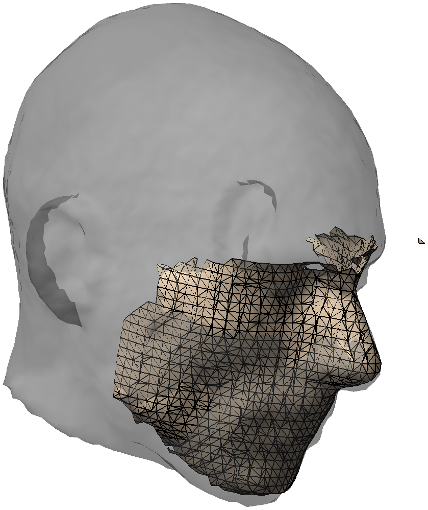
Figure: 3D scan of the face aligned with the MRI-derived face.

Interactive alignment of the helmet with the template helmet

We can also interactively align the helmet from the 3D scan with the template helmet. For this we use the 3D model of the actual FieldLine helmet. The template helmet only contains the rim around the face.

helmet_rim = ft_read_headshape('fieldlinebeta2_helmet_rim.mat');
helmet_rim.coordsys = 'ras';

To achieve a reasonably good alignment between the scanned helmet and the 3D model helmet rim, the following values can be specified (without clicking the ‘apply’ button in between) for the rotation: [20 -2 0], and for the translation: [-0.003 0.065 -0.045]. Note that the units are expressed in ‘m’.

cfg = [];
cfg.method = 'interactive';
cfg.headshape = helmet_rim;
cfg.meshstyle = {'edgecolor', 'none', 'facecolor', [1 0.5 0.5]};
scan_helmet_aligned = ft_meshrealign(cfg, scan_helmet);

figure; hold on;
ft_plot_mesh(model_helmet_rim, 'edgecolor', 'none', 'facecolor', [0.5 0.5 1], 'facealpha', 0.4);
ft_plot_mesh(scan_helmet_aligned, 'edgecolor', 'none', 'facecolor', [1 0.5 0.5], 'facealpha', 0.4);
view([145 10]);
lighting gouraud
material dull
light

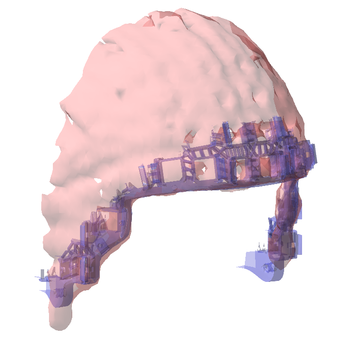
Figure: 3D scan of the helmet aligned with the 3D model of the actual FieldLine helmet.

Calculation of the transformation matrix

The three objects (the optical 3D scan, the face from the MRI and the template helmet) are initially all expressed in different coordinate systems. In the previous steps we have determined two pairwise transformations, which can be combined and used to align each of the objects to any other object.

Now we can use the transformation that align the face from the 3D scan with the face from the anatomical MRI and the transformation that align the helmet from the 3D scan with the sensors to calculate the transformation that aligns the sensors with the anatomical MRI.

transform_scan2helmet = scan_helmet_aligned.cfg.transform;
transform_scan2face   = scan_face_aligned.cfg.transform;
transform_helmet2face = transform_scan2face/transform_scan2helmet;

These are all expressed as 4x4 matrices that represent homogenous coordinate transformations.

Apply the transformation matrix to the sensors

The transformation matrix transform_helmet2face can now be used to update the sensor definition, which aligns the sensors with head-based coordinate system.

fieldlinebeta2 = ft_read_sens('fieldlinebeta2.mat');  % from fieldtrip/template/grad
fieldlinebeta2.coordsys = 'ras';

% align the sensors to the head
fieldlinebeta2_head = ft_transform_geometry(transform_helmet2face, fieldlinebeta2);

figure; hold on;
ft_plot_sens(fieldlinebeta2_head);
ft_plot_headshape(mri_face, 'facecolor', [0.5 0.5 1], 'facealpha', 0.4, 'edgecolor', 'none');
view([125 10]);
lighting gouraud
material dull
light

Figure: sensors aligned with the anatomical MRI.

We can see that the participant was not positioned very high in the FieldLine helmet. This particular example was acquired to demonstrate the coregistration, not for an actual OPM MEG measurement.

Coregistration using the sensors following the head shape

This is specific for the FieldLine smart helmet.

More info to follow: stay tuned!

Coregistration of individually designed 3D printed helmets

The coregistration of individually designed 3D printed helmets is mostly done during the design phase, as the helmet is designed around a geometrical model of the head surface.

The procedure for this consists of the following steps:

• Import the anatomical MRI from the participant with ft_read_mri, use ft_volumerealign to align and ft_volumesegment to segment the scalp surface. Then use **ft_prepare_mesh to construct a triangulated surface.
• Alternatively to starting with an MRI, you can also start with a 3D scan of the participants head. while wearing a swimming cap or similar to press down the hair. In that case you proceed with ft_read_headshape, ft_meshrealign to align, and ft_defacemesh to remove unwanted parts from the mesh, like the shoulders and/or the face.
• You export the mesh as an STL file using ft_write_headshape and import it in your favourite 3D design software like Fusion360, Solidworks or Blender. From there it is up to you to design the helmet, including the OPM sensor holders.

Summary and suggested further reading

This tutorial gave an introduction on the coregistration of OPM data, specifically dealing with OPM data that has been collected with the sensors positioned in in a known helmet configuration.

You may want to continue with the more general tutorials on processing MEG (and EEG) data, or have a look at the system specific details for the OPM data that you are working with. Also, you may want to proceed with the OPM preprocessing tutorial.

Furthermore, you can explore other pages that deal with OPMs:

• Getting started with Cerca OPM data
• Coregistration of Optically Pumped Magnetometer (OPM) data
• Getting started with FieldLine OPM data
• Template 2-D layouts for plotting
• Getting started with OPM data recorded at the FIL
• Preprocessing of Optically Pumped Magnetometer (OPM) data